All in One View
Content from Overview of Google Cloud for Machine Learning and AI
Last updated on 2026-03-04 | Edit this page
Estimated time: 12 minutes
Overview
Questions
- Why would I run ML/AI experiments in the cloud instead of on my laptop or an HPC cluster?
- What does GCP offer for ML/AI, and how is it organized?
- What is the “notebook as controller” pattern?
Objectives
- Identify when cloud compute makes sense for ML/AI work.
- Describe what GCP and Vertex AI provide for ML/AI researchers.
- Explain the notebook-as-controller pattern used throughout this workshop.
Why run ML/AI in the cloud?
You have ML/AI code that works on your laptop. But at some point you need more — a bigger GPU (or multiple GPUs), a dataset that won’t fit on disk, or the ability to run dozens of training experiments overnight. You could invest in local hardware or compete for time on a shared HPC cluster, but cloud platforms let you rent exactly the hardware you need, for exactly as long as you need it, and then shut it down.
Cloud vs. university HPC clusters
Most universities offer shared HPC clusters with GPUs. These are excellent resources — but they have tradeoffs worth understanding:
| Factor | University HPC | Cloud (GCP) |
|---|---|---|
| Cost | Free or subsidized | Pay per hour |
| GPU availability | Shared queue; wait times during peak periods and per-job runtime limits (often 24–72 hrs) that may require checkpointing long training runs | On-demand (subject to quota); jobs run as long as needed |
| Hardware variety | Fixed hardware refresh cycle (3–5 years) | Latest GPUs available immediately (A100, H100, L4) |
| Scaling | Limited by cluster size | Spin up hundreds of jobs in parallel |
| Multi-GPU / NVLink | Sometimes available, depends on cluster | Available on demand (e.g., A2/A3 instances with NVLink-connected multi-GPU nodes) — essential for training, fine-tuning, or serving large LLMs that don’t fit in a single GPU’s memory |
| Job orchestration | Writing scheduler scripts, packaging environments, and wiring up parallel job arrays can take days of refactoring | A few SDK calls: define a job, set hardware, call
.run() — parallelism (e.g., tuning trials) is built in |
| Software environment | Module system; some clusters support Apptainer/Singularity containers — research computing staff can often help with setup | Vertex AI provides prebuilt
containers for common ML frameworks (PyTorch, XGBoost, TensorFlow);
add extra packages via a requirements list, or bring your
own Docker image for full control |
| Power & cooling | Paid for by the university; campus data centers often spend nearly as much energy on cooling as on the computers themselves | Google’s data centers are roughly twice as energy-efficient as a typical campus facility — and power, cooling, and hardware failures are their problem, not yours |
The short version: use your university cluster when it has the hardware you need and the queue isn’t blocking you. Use the cloud when you need hardware your cluster doesn’t have, need to scale beyond what the queue allows, or need a specific software environment you can’t easily get on-campus.
Many researchers use both — develop and test on HPC, then scale to cloud for large experiments or specialized hardware. This workshop teaches the cloud side of that workflow.
When does model size justify cloud compute?
Not every model needs cloud hardware. Here’s a rough guide:
| Model scale | Parameters | Example models | Where to run |
|---|---|---|---|
| Small | < 10M | Logistic regression, small CNNs, XGBoost | Laptop or HPC — cloud adds overhead without much benefit |
| Medium | 10M–500M | ResNets, BERT-base, mid-sized transformers | HPC with a single GPU (RTX 2080 Ti, L40) or cloud (T4, L4) |
| Large | 500M–10B | GPT-2, LLaMA-7B, fine-tuning large transformers | HPC with A100 (40/80 GB) or cloud — both work well |
| Very large | 10B–70B | LLaMA-70B, Mixtral | HPC with H100/H200 (80–141 GB) or cloud multi-GPU nodes |
| Frontier | 70B+ | GPT-4-scale, multi-expert models | Cloud — requires multi-node clusters beyond what most HPC queues offer |
CHTC’s GPU Lab covers more than you might think. The GPU Lab includes A100s (40 and 80 GB), H100s (80 GB), and H200s (141 GB) — enough VRAM to run inference or fine-tune models up to ~70B parameters on a single GPU with quantization. For many UW researchers, this hardware handles “large model” workloads without needing cloud. Jobs have time limits (12 hrs for short, 24 hrs for medium, 7 days for long jobs), so plan your training runs accordingly.
Cloud becomes the clear choice when you need interconnected multi-GPU nodes (NVLink) for large distributed training, hardware beyond what the GPU Lab queue offers, or when queue wait times are blocking a deadline.
A note on cloud costs
Cloud computing is not free, but it’s worth putting costs in context:
-
Hardware is expensive and ages fast. A single A100
GPU costs ~
$15,000and is outdated within a few years. Cloud lets you rent the latest hardware by the hour. - You pay only for what you use. Stop a VM and the meter stops — valuable for bursty research workloads.
- Managed services save development time. You don’t have to build DAGs, write scheduling logic, package custom containers, or maintain orchestration infrastructure — GCP handles that plumbing so you can focus on the ML.
- Budgets and alerts keep you safe. GCP billing dashboards and budget alerts help prevent surprise bills. We cover cleanup in Episode 9.
The key habit: choose the right machine size, stop resources when idle, and monitor spending. We’ll reinforce this throughout.
For UW-Madison researchers
UW-Madison offers reduced-overhead cloud billing, NIH STRIDES
discounts, Google Cloud research credits (up to $5,000),
free on-campus GPUs via CHTC,
and dedicated support from the Public Cloud Team. See the
UW-Madison Cloud Resources
page for details.
Google Cloud Platform (GCP) is one of several clouds that supports this. The rest of this episode explains what GCP offers for ML/AI and how the pieces fit together.
What GCP provides for ML/AI
GCP gives you three things that matter for applied ML/AI research:
Flexible compute. You pick the hardware that fits your workload:
- CPUs for lightweight models, preprocessing, or feature engineering.
- GPUs (NVIDIA T4, L4, V100, A100, H100) for training deep learning models. For help choosing, see Compute for ML.
- TPUs (Tensor Processing Units) — Google’s custom hardware for matrix-heavy workloads. TPUs work best with TensorFlow and JAX; PyTorch support is improving but still less mature.
Scalable storage. Google Cloud Storage (GCS) buckets give you a place to store datasets, scripts, and model artifacts that any job or notebook can access. Think of it as a shared filesystem for your project.
Managed ML/AI services. Vertex AI is Google’s ML/AI platform. It wraps compute, storage, and tooling into a set of services designed for ML/AI workflows — managed notebooks, training jobs, hyperparameter tuning, model hosting, and access to foundation models like Gemini.
How the pieces fit together: Vertex AI
Google Cloud has many products and brand names. Here are the ones you’ll use in this workshop and how they relate:
| Term | What it is |
|---|---|
| GCP | Google Cloud Platform — the overall cloud: compute, storage, networking. |
| Vertex AI | Google’s ML platform — notebooks, training jobs, tuning, model hosting. Everything below lives under this umbrella. |
| Workbench | Managed Jupyter notebooks that run on a Compute Engine VM. Your interactive environment. |
| Training & tuning jobs | How you run code on Vertex AI hardware. You submit a script and a
machine spec; Vertex AI provisions the VM, runs it, and shuts it down.
The SDK offers several flavors — CustomTrainingJob (Ep
4–5), HyperparameterTuningJob (Ep 6) — and the CLI
equivalent is gcloud ai custom-jobs (Ep 8). |
| Cloud Storage (GCS) | Object storage for files. Similar to AWS S3. |
| Compute Engine | Virtual machines you configure with CPUs, GPUs, or TPUs. Workbench and training jobs run on Compute Engine under the hood. |
| Gemini | Google’s family of large language models, accessed through the Vertex AI API. |
For a full list of terms, see the Glossary.
The notebook-as-controller pattern
The central idea of this workshop is simple: you work in a lightweight Vertex AI Workbench notebook — a small, cheap VM — and use the Vertex AI Python SDK to dispatch work to managed services. The notebook itself does not run heavy compute. Instead, it orchestrates:
- Training jobs (Eps 4–5) — run your script on auto-provisioned GPU hardware, then shut down when complete.
- Hyperparameter tuning jobs (Ep 6) — search a parameter space across parallel trials and return the best configuration.
- Cloud Storage (Ep 3) — shared persistent storage for datasets, model artifacts, logs, and results.
- Gemini API (Ep 7) — embeddings and generation for Retrieval-Augmented Generation (RAG) pipelines.
All of these are accessed via SDK calls from the notebook. This keeps costs low (the notebook VM stays small) and keeps your work reproducible (each job is a clean, logged run on dedicated hardware).

Console, notebooks, or CLI — your choice
This workshop uses the GCP web console and
Workbench notebooks for most tasks because they’re
visual and easy to follow for beginners. But nearly everything we do can
also be done from the gcloud command-line
tool — submitting training jobs, managing buckets, checking
quotas. Episode 8 covers the CLI
equivalents. If you prefer terminal-based workflows or need to automate
jobs in scripts and CI/CD pipelines, that episode shows you how.
One important caveat: whether you use the console, notebooks, or CLI, resources you create (VMs, training jobs, endpoints) keep running and billing until you explicitly stop them. There’s no automatic shutdown. We cover cleanup habits in Episode 9, but the short version is: always check for running resources before you walk away.
Your current setup
Think about how you currently run ML experiments:
- What hardware do you use — laptop, HPC cluster, cloud?
- What’s the biggest infrastructure pain point in your workflow (GPU access, environment setup, data transfer, cost)?
- What would you most like to offload to a managed service?
Take 3–5 minutes to discuss with a partner or share in the workshop chat.
- Cloud platforms let you rent hardware on demand instead of buying or waiting for shared resources.
- GCP organizes its ML/AI services under Vertex AI — notebooks, training jobs, tuning, and model hosting.
- The notebook-as-controller pattern keeps your notebook cheap while offloading heavy training to dedicated Vertex AI jobs.
- Everything in this workshop can also be done from the
gcloudCLI (Episode 8).
Content from Notebooks as Controllers
Last updated on 2026-03-05 | Edit this page
Estimated time: 30 minutes
Overview
Questions
- How do you set up and use Vertex AI Workbench notebooks for machine
learning tasks?
- How can you manage compute resources efficiently using a “controller” notebook approach in GCP?
Objectives
- Describe how Vertex AI Workbench notebooks fit into ML/AI workflows on GCP.
- Set up a Jupyter-based Workbench Instance as a lightweight controller to manage compute tasks.
- Configure a Workbench Instance with appropriate machine type, labels, and idle shutdown for cost-efficient orchestration.
Setting up our notebook environment
Google Cloud Workbench provides JupyterLab-based environments that can be used to orchestrate ML/AI workflows. In this workshop, we will use a Workbench Instance—the recommended option going forward, as other Workbench environments are being deprecated.
Workbench Instances come with JupyterLab 3 pre-installed and are configured with GPU-enabled ML frameworks (TensorFlow, PyTorch, etc.), making it easy to start experimenting without additional setup. Learn more in the Workbench Instances documentation.
Using the notebook as a controller
The notebook instance functions as a controller to manage
more resource-intensive tasks. By selecting a modest machine type (e.g.,
n2-standard-2), you can perform lightweight operations
locally in the notebook while using the Vertex AI Python
SDK to launch compute-heavy jobs on larger machines (e.g.,
GPU-accelerated) when needed.
This approach minimizes costs while giving you access to scalable infrastructure for demanding tasks like model training, batch prediction, and hyperparameter tuning.
One practical advantage of Workbench notebooks:
authentication is automatic. A Workbench VM inherits
the permissions of its attached service account, so calls to Cloud
Storage, Vertex AI, and the Gemini API work with no extra credential
setup — no API keys or login commands needed. If you later run the same
code from your laptop or an HPC cluster, you’ll need to set up
credentials separately (see the GCP authentication
docs). (Prefer working from a terminal? Episode 8: CLI Workflows covers how to
do everything in this workshop using gcloud commands
instead of notebooks.)
We will follow these steps to create our first Workbench Instance:
1. Navigate to Workbench
- Open the Google Cloud Console (console.cloud.google.com) — this is the web dashboard where you manage all GCP resources. Search for “Workbench.”
- Click the “Instances” tab (this is the supported path going forward).
2. Create a new Workbench Instance
Initial settings
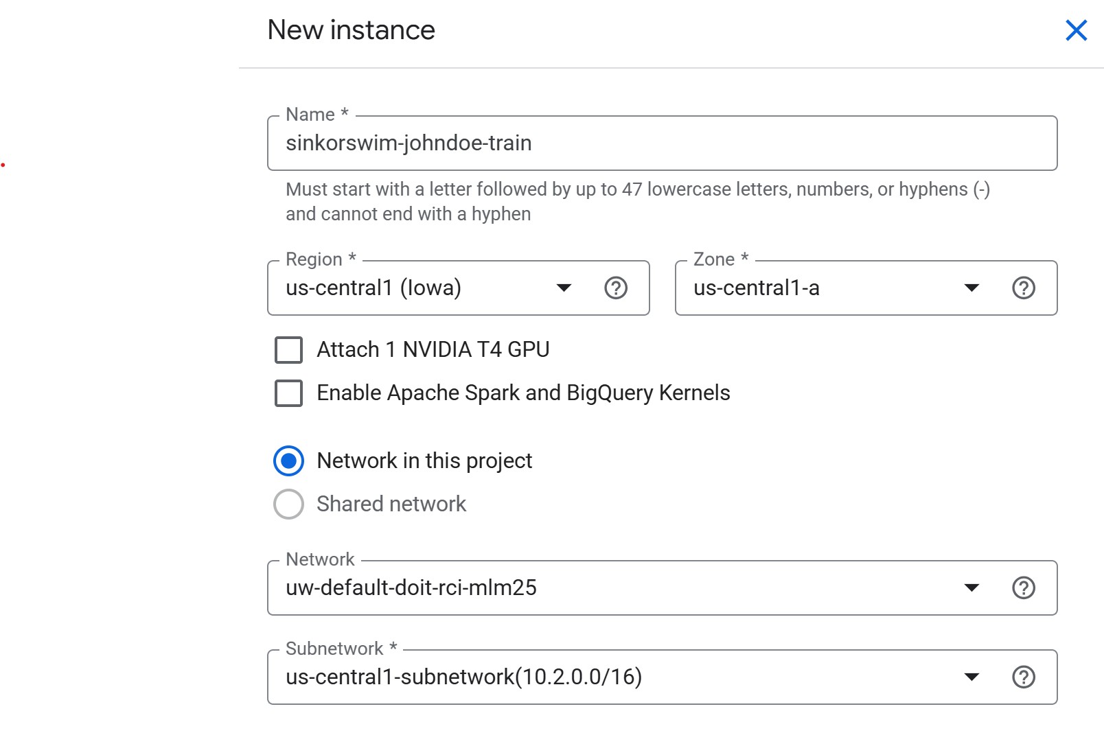
- Click Create New near the top of the Workbench page
-
Name: Use the convention
lastname-purpose(e.g.,doe-workshop). GCP resource names only allow lowercase letters, numbers, and hyphens. We’ll use a single instance for training, tuning, RAG, and more, soworkshopis a good general-purpose label. -
Region: Select
us-central1. When we create a storage bucket in Episode 3, we’ll use the same region — keeping compute and storage co-located avoids cross-region transfer charges and keeps data access fast. -
Zone:
us-central1-a(or another zone inus-central1, like-bor-c)- If capacity or GPU availability is limited in one zone, switch to another zone in the same region.
-
NVIDIA T4 GPU: Leave unchecked for now
- We will request GPUs for training jobs separately. Attaching here increases idle costs.
-
Apache Spark and BigQuery Kernels: Leave unchecked
- BigQuery kernels let you run SQL analytics directly in a notebook, but we won’t need them in this workshop. Leave unchecked to avoid pulling extra container images.
- Network in this project: If you’re working in a shared workshop environment, select the network provided by your administrator (shared environments typically do not allow using external or default networks). If using a personal GCP project, the default network is fine.
-
Network / Subnetwork: Leave as pre-filled.
Advanced settings: Details (tagging)
-
IMPORTANT: Open the “Advanced options” menu next.
-
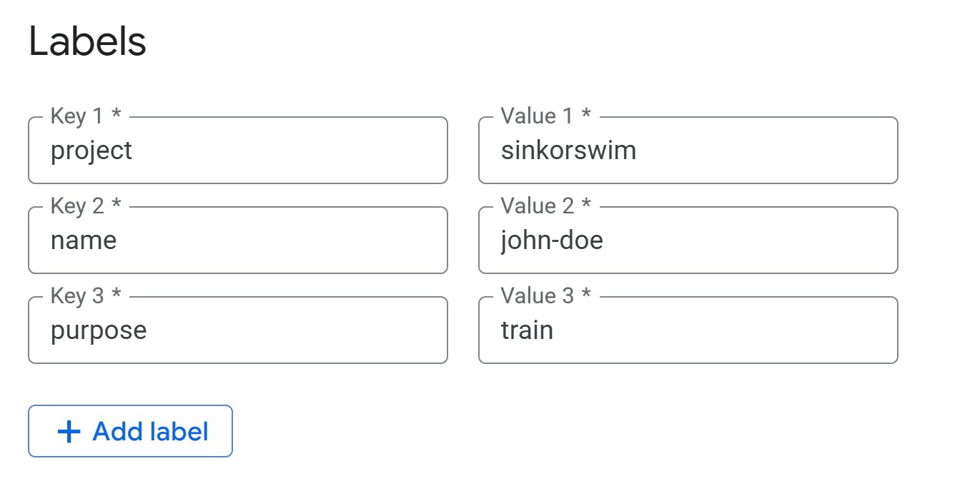
Labels (required for cost tracking): Under the
Details menu, add the following tags (all lowercase) so that you can
track the total cost of your activity on GCP later:
name = firstname-lastnamepurpose = workshop
-
Labels (required for cost tracking): Under the
Details menu, add the following tags (all lowercase) so that you can
track the total cost of your activity on GCP later:
Advanced Settings: Environment
Leave environment settings at their defaults for this workshop.
Workbench uses JupyterLab 3 by default with NVIDIA GPU drivers, CUDA,
and common ML frameworks preinstalled. For future reference, you can
optionally select JupyterLab 4, provide a custom Docker image, or
specify a post-startup script (gs://path/to/script.sh) to
auto-configure the instance at boot.
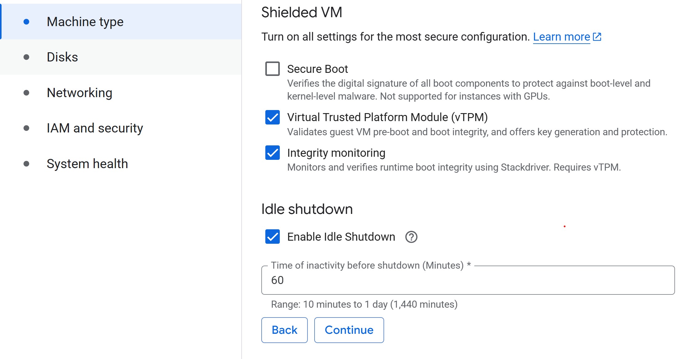
Advanced settings: Machine Type
-
Machine type: Select a small machine (e.g.,
n2-standard-2, ~$0.07/hr) to act as the controller.- This keeps costs low while you delegate heavy lifting to training jobs.
- For guidance on common machine types and their costs, see Compute for ML. For help deciding when you need cloud hardware at all, see When does model size justify cloud compute? in Episode 1.
- Set idle shutdown: To save on costs when you aren’t doing anything in your notebook, lower the default idle shutdown time to 60 (minutes).
Advanced Settings: Disks
Leave disk settings at their defaults for this workshop. Each Workbench Instance has two disks: a boot disk (100 GB — holds the OS and libraries) and a data disk (150 GB default — holds your datasets and outputs). Both use Balanced Persistent Disks. Keep “Delete to trash” unchecked so deleted files free space immediately.
Rule of thumb: allocate ≈ 2× your dataset size for
the data disk, and keep bulk data in Cloud Storage (gs://)
rather than on local disk — PDs cost ~ $0.10/GB/month vs. ~
$0.02/GB/month for Cloud Storage.
Disk sizing and cost details
- Boot disk: Rarely needs resizing. Increase to 150–200 GB only for large custom environments or multiple frameworks.
- Data disk: Use SSD PD only for high-I/O workloads. Disks can be resized anytime without downtime, so start small and expand when needed.
-
Cost comparison: A 200 GB dataset costs ~
$24/month on a PD but only ~$5/month in Cloud Storage. - Pricing: Persistent Disk pricing · Cloud Storage pricing
Create notebook
- Click Create to create the instance. Provisioning typically takes 3–5 minutes. You’ll see the status change from “Provisioning” to “Active” with a green checkmark. While waiting, work through the challenges below.
Challenge 1: Notebook Roles
Your university provides different compute options: laptops, on-prem HPC, and GCP.
- What role does a Workbench Instance notebook play compared to an HPC login node or a laptop-based JupyterLab?
- Which tasks should stay in the notebook (lightweight control, visualization) versus being launched to larger cloud resources?
The notebook serves as a lightweight control plane.
- Like an HPC login node, it is not meant for heavy computation.
- Suitable for small preprocessing, visualization, and orchestrating jobs.
- Resource-intensive tasks (training, tuning, batch jobs) should be submitted to scalable cloud resources (GPU/large VM instances) via the Vertex AI SDK.
Challenge 2: Controller Cost Estimate
Your controller notebook uses an n2-standard-2 instance
(~ $0.07/hr — see Compute for
ML for other common machine types and costs).
- Estimate the monthly cost if you use it 8 hours/day, 5 days/week, with idle shutdown enabled.
- Compare that to leaving it running 24/7 for the same month.
-
With idle shutdown: 8 hrs × 5 days × 4 weeks = 160
hrs → 160 ×
$0.07≈$11.20/month -
Running 24/7: 24 hrs × 30 days = 720 hrs → 720 ×
$0.07≈$50.40/month - Idle shutdown saves you ~
$39/month on a single small controller instance. The savings are even larger for bigger machine types.
Managing your instance
You don’t have to wait for idle shutdown — you can manually stop your instance anytime from the Workbench Instances list by selecting the checkbox and clicking Stop. To resume work, click Start. You only pay for compute while the instance is running (disk charges continue while stopped).
To permanently remove an instance, select it and click Delete. Full cleanup is covered in Episode 9.
Managing training and tuning with the controller notebook
In the following episodes, we will use the Vertex AI Python
SDK (google-cloud-aiplatform) from this notebook
to submit compute-heavy tasks on more powerful machines. Examples
include:
- Training a model on a GPU-backed instance.
- Running hyperparameter tuning jobs managed by Vertex AI.
Here’s how the notebook, jobs, and storage connect:

This pattern keeps costs low by running your notebook on a modest VM while only incurring charges for larger resources when they are actively in use.
You don’t need a notebook to use Vertex AI
We start with Vertex AI Workbench notebooks because they give you authenticated access to buckets, training jobs, and other GCP services out of the box — no credential setup required. The Console UI also lets you see and manage running jobs directly, which matters when you’re learning: accidentally submitting a duplicate training job is easy to spot and cancel in the Console, harder to notice from a terminal.
Episode 8 introduces the
gcloud CLI once these concepts are
familiar. Notebooks are not required for any of the
workflows covered here — everything we do through the Python SDK can
also be done from:
- A plain Python script run from your terminal or an HPC scheduler.
- The
gcloudCLI (e.g.,gcloud ai custom-jobs create ...). - A CI/CD pipeline (GitHub Actions, Cloud Build, etc.).
The real work happens in the training scripts and SDK calls — the notebook is just a convenient starting point.
Troubleshooting
-
VM stuck in “Provisioning” for more than 5 minutes?
Try deleting the instance and re-creating it in a different zone within
the same region (e.g.,
us-central1-binstead ofus-central1-a). - Instance stopped unexpectedly? Check the idle shutdown setting — it may have timed out. Restart from the Instances list by clicking Start.
- Can’t see the project or get permission errors? Ensure you’re signed into the correct Google account and that IAM permissions have propagated (this can take a few minutes after initial setup).
Load pre-filled Jupyter notebooks
Once your instance shows as “Active” (green checkmark), click Open JupyterLab. From the Launcher, select Python 3 (ipykernel) under Notebook to create a new notebook — we don’t need the TensorFlow or PyTorch kernels yet, as those are used in later episodes for training jobs.
Run the following command to clone the lesson repository. This contains pre-filled notebooks for each episode and the training scripts we’ll use later, so you won’t need to write boilerplate code from scratch.
Then, navigate to
/Intro_GCP_for_ML/notebooks/03-Data-storage-and-access.ipynb
to begin the next episode.
- Use a small Workbench Instance as a controller — delegate heavy training to Vertex AI jobs.
- Workbench VMs inherit service account permissions automatically, simplifying authentication.
- Choose the same region for your Workbench Instance and storage bucket to avoid extra transfer costs.
- Apply labels to all resources for cost tracking, and enable idle auto-stop to avoid surprise charges.
Content from Data Storage and Access
Last updated on 2026-03-05 | Edit this page
Estimated time: 50 minutes
Overview
Questions
- How can I store and manage data effectively in GCP for Vertex AI workflows?
- What are the advantages of Google Cloud Storage (GCS) compared to local or VM storage for machine learning projects?
- How can I load data from GCS into a Vertex AI Workbench notebook?
Objectives
- Explain data storage options in GCP for machine learning projects.
- Set up a GCS bucket and upload data.
- Read data directly from a GCS bucket into memory in a Vertex AI notebook.
- Monitor storage usage and estimate costs.
- Upload new files from the Vertex AI environment back to the GCS bucket.
ML/AI projects rely on data, making efficient storage and management essential. Google Cloud offers several storage options, but the most common for ML/AI workflows are Virtual Machine (VM) disks and Google Cloud Storage (GCS) buckets.
Consult your institution’s IT before handling sensitive data in GCP
As with AWS, do not upload restricted or sensitive data to GCP services unless explicitly approved by your institution’s IT or cloud security team. For regulated datasets (HIPAA, FERPA, proprietary), work with your institution to ensure encryption, restricted access, and compliance with policies.
Options for storage: VM Disks or GCS
What is a VM disk?
A VM disk is the storage volume attached to a Compute Engine VM or a Vertex AI Workbench notebook. It can store datasets and intermediate results, but it is tied to the lifecycle of the VM.
When to store data directly on a VM disk
- Useful for small, temporary datasets processed interactively.
- Data persists if the VM is stopped, but storage costs continue as long as the disk exists.
- Not ideal for collaboration, scaling, or long-term dataset storage.
Limitations of VM disk storage
- Scalability: Limited by disk size quota.
- Sharing: Harder to share across projects or team members.
- Cost: More expensive per GB compared to GCS for long-term storage.
What is a GCS bucket?
For most ML/AI workflows in GCP, Google Cloud Storage (GCS)
buckets are recommended. A GCS bucket is a container in
Google’s object storage service where you can store an essentially
unlimited number of files. Data in GCS can be accessed from Vertex AI
training jobs, Workbench notebooks, and other GCP services using a
GCS URI (e.g.,
gs://your-bucket-name/your-file.csv). Think of GCS URIs as
cloud file paths — you’ll use them throughout the workshop to reference
data in training scripts, notebooks, and SDK calls.
Benefits of using GCS (recommended for ML/AI workflows)
- Separation of storage and compute: Data remains available even if VMs or notebooks are deleted.
- Easy sharing: Buckets can be accessed by collaborators with the right IAM roles.
- Integration with Vertex AI and BigQuery: Read and write data directly using other GCP tools.
- Scalability: Handles datasets of any size without disk limits.
- Cost efficiency: Lower cost than persistent disks (VM storage) for long-term storage.
- Data persistence: Durable and highly available across regions.
- Filesystem mounting: GCS buckets can be mounted as local directories using Cloud Storage FUSE, making them accessible like regular filesystems for tools that expect local file paths.
Creating a GCS bucket
1. Sign in to Google Cloud Console
- Go to console.cloud.google.com and log in with your credentials.
- Select your project from the project dropdown at the top of the page. If you’re using the shared workshop project, the instructor will provide the project name.
3. Create a new bucket
Click Create bucket and configure the following settings:
Bucket name: Enter a globally unique name using the convention
lastname-dataname(e.g.,doe-titanic).-
Labels: Add cost-tracking labels (same keys you used for the Workbench Instance in Episode 2, plus a
datasettag):name = firstname-lastnamepurpose = workshopdataset = titanic
In shared accounts, labels are mandatory.
Location: Choose Region →
us-central1(same region as your compute to avoid egress charges).Storage class: Standard (best for active ML/AI workflows).
Access control: Uniform (simpler IAM-based permissions).
Protection: Leave default soft delete enabled; skip versioning and retention policies.
Click Create if everything looks good.
4. Upload files to the bucket
- If you haven’t yet, download the data for this workshop (Right-click
→ Save as): data.zip
- Extract the zip folder contents (Right-click → Extract all on Windows; double-click on macOS).
- The zip contains the Titanic dataset — passenger information (age, class, fare, etc.) with a survival label. This is a classic binary classification task we’ll use for training in later episodes.
- In the bucket dashboard, click Upload Files.
- Select your Titanic CSVs (
titanic_train.csvandtitanic_test.csv) and upload.
Note the GCS URI for your data After uploading,
click on a file and find its gs:// URI (e.g.,
gs://doe-titanic/titanic_test.csv). This URI will be used
to access the data in your notebook.
Adjust bucket permissions
Your bucket exists, but your notebooks and training jobs don’t automatically have permission to use it. GCP follows the principle of least privilege — services only get the access you explicitly grant. In this section we’ll find the service account that Vertex AI uses and give it the right roles on your bucket.
Check your project ID
First, confirm which project your notebook is connected to. Run this cell in your Workbench notebook:
Copy the output — you’ll paste it into Cloud Shell commands below.
These commands run in Cloud Shell, not in a notebook
Open Cloud Shell — a browser-based terminal built into the Google Cloud Console (click the >_ icon in the top-right toolbar). Copy the commands below and paste them into that terminal.
Set your project
If Cloud Shell doesn’t already know your project, set it first:
Replace YOUR_PROJECT_ID with the project ID you copied
above. For the shared MLM25 workshop the project ID is
doit-rci-mlm25-4626.
Find your service account
When you create a GCP project, Google automatically provisions a Compute Engine default service account. This is the identity that Vertex AI Workbench notebooks and training jobs use when they call other GCP services (like Cloud Storage). By default this account may not have access to your bucket, so we need to grant it the right IAM roles explicitly.
First, look up the service account email:
SH
gcloud iam service-accounts list --filter="displayName:Compute Engine default service account" --format="value(email)"This will return an email like
123456789-compute@developer.gserviceaccount.com. Copy it —
you’ll paste it into the commands below.
Grant permissions
Now we give that service account the ability to read from and write to your bucket. Without these roles, your notebooks would get “Access Denied” errors when trying to load training data or save model artifacts.
Replace YOUR_BUCKET_NAME and
YOUR_SERVICE_ACCOUNT, then run:
SH
# objectViewer — lets notebooks READ data (e.g., load CSVs for training)
gcloud storage buckets add-iam-policy-binding gs://YOUR_BUCKET_NAME \
  --member="serviceAccount:YOUR_SERVICE_ACCOUNT" \
  --role="roles/storage.objectViewer"

# objectCreator — lets training jobs WRITE outputs (e.g., saved models, logs)
gcloud storage buckets add-iam-policy-binding gs://YOUR_BUCKET_NAME \
  --member="serviceAccount:YOUR_SERVICE_ACCOUNT" \
  --role="roles/storage.objectCreator"

# objectAdmin — adds OVERWRITE and DELETE (only needed if you want to
# re-run jobs that replace existing files or clean up old artifacts)
gcloud storage buckets add-iam-policy-binding gs://YOUR_BUCKET_NAME \
  --member="serviceAccount:YOUR_SERVICE_ACCOUNT" \
  --role="roles/storage.objectAdmin"
gcloud storage
vs. gsutil
Older tutorials often reference gsutil for Cloud Storage
operations. Google now recommends gcloud storage as the
primary CLI. Both work, but gcloud storage is actively
maintained and consistent with the rest of the gcloud
CLI.
Data transfer & storage costs
GCS costs are based on three things: storage class (how you store data), data transfer (moving data in or out of GCP), and operations (API requests). Operations are the individual actions your code performs against Cloud Storage — every time a notebook reads a file or a training job writes a model, that’s an API request.
-
Standard storage: ~
$0.02per GB per month inus-central1. - Uploading data (ingress): Free.
-
Downloading data out of GCP (egress): ~
$0.12per GB. -
Cross-region access: ~
$0.01–$0.02per GB within North America. -
GET requests (reading/downloading objects): ~
$0.004per 10,000 requests. -
PUT/POST requests (creating/uploading objects): ~
$0.05per 10,000 requests. - Deleting data: Free (but Nearline/Coldline/Archive early-deletion fees apply).
For detailed pricing, see GCS Pricing Information.
Challenge 1: Estimating Storage Costs
1. Estimate the total cost of storing 1 GB in GCS Standard storage (us-central1) for one month assuming: - Dataset read from the bucket 100 times within GCP (e.g., each training or tuning run fetches the data via a GET request — this stays inside Google’s network, so no egress charge) - Data is downloaded once out of GCP to your laptop at the end of the project (this does incur an egress charge)
2. Repeat the above calculation for datasets of 10 GB, 100 GB, and 1 TB (1024 GB).
Hints: Storage $0.02/GB/month, Egress
$0.12/GB, GET requests negligible at this scale.
-
1 GB: Storage
$0.02+ Egress$0.12=$0.14 -
10 GB:
$0.20+$1.20=$1.40 -
100 GB:
$2.00+$12.00=$14.00 -
1 TB:
$20.48+$122.88=$143.36
Accessing data from your notebook
Now that our bucket is set up, let’s use it from the Workbench notebook you created in the previous episode.
If you haven’t already cloned the repository, open JupyterLab from
your Workbench Instance and run
!git clone https://github.com/qualiaMachine/Intro_GCP_for_ML.git.
Then navigate to
/Intro_GCP_for_ML/notebooks/03-Data-storage-and-access.ipynb.
Set up GCP environment
If you haven’t already, initialize the storage client (same code from
the permissions section earlier). The storage.Client() call
creates a connection using the credentials already attached to your
Workbench VM.
Reading data directly into memory
The code below downloads a CSV from your bucket and loads it into a
pandas DataFrame. The blob.download_as_bytes() call pulls
the file contents as raw bytes, and io.BytesIO wraps those
bytes in a file-like object that pd.read_csv can read — no
temporary file on disk needed.
PYTHON
import pandas as pd
import io

bucket_name = "doe-titanic" # ADJUST to your bucket's name

bucket = client.bucket(bucket_name)
blob = bucket.blob("titanic_train.csv")
train_data = pd.read_csv(io.BytesIO(blob.download_as_bytes()))
print(train_data.shape)
train_data.head()
The Titanic dataset contains passenger information (age, class, fare, etc.) and a binary survival label — we’ll train a classifier on this data in Episode 4.
Alternative: reading directly with pandas
Vertex AI Workbench comes with gcsfs pre-installed,
which lets pandas read GCS URIs directly — no BytesIO
conversion needed:
This is convenient for quick exploration. We use the
storage.Client approach above because it gives you more
control (listing blobs, checking sizes, uploading), which you’ll need in
the sections that follow.
Common errors
-
Forbidden (403)— Your service account lacks permission. Revisit the Adjust bucket permissions section above. -
NotFound (404)— The bucket name or file path is wrong. Double-checkbucket_nameand the blob path withclient.list_blobs(bucket_name). -
DefaultCredentialsError— The notebook cannot find credentials. Make sure you are running on a Vertex AI Workbench Instance (not a local machine).
Monitoring storage usage and costs
It’s good practice to periodically check how much storage your bucket is using. The code below sums up all object sizes.
PYTHON
total_size_bytes = 0
bucket = client.bucket(bucket_name)

for blob in client.list_blobs(bucket_name):
    total_size_bytes += blob.size

total_size_mb = total_size_bytes / (1024**2)
print(f"Total size of bucket '{bucket_name}': {total_size_mb:.2f} MB")
PYTHON
storage_price_per_gb = 0.02   # $/GB/month for Standard storage
egress_price_per_gb = 0.12    # $/GB for internet egress (same-region transfers are free)
total_size_gb = total_size_bytes / (1024**3)

monthly_storage = total_size_gb * storage_price_per_gb
egress_cost = total_size_gb * egress_price_per_gb

print(f"Bucket size: {total_size_gb:.4f} GB")
print(f"Estimated monthly storage cost: ${monthly_storage:.4f}")
print(f"Estimated annual storage cost:  ${monthly_storage*12:.4f}")
print(f"One-time full download (egress) cost: ${egress_cost:.4f}")
Writing output files to GCS
PYTHON
# Create a sample file locally on the notebook VM
file_path = "/home/jupyter/Notes.txt"
with open(file_path, "w") as f:
    f.write("This is a test note for GCS.")
PYTHON
bucket = client.bucket(bucket_name)
blob = bucket.blob("docs/Notes.txt")
blob.upload_from_filename(file_path)
print("File uploaded successfully.")
List bucket contents:
Challenge 2: Read and explore the test dataset
Read titanic_test.csv from your GCS bucket and display
its shape. How does the test set compare to the training set in size and
columns?
PYTHON
blob = client.bucket(bucket_name).blob("titanic_test.csv")
test_data = pd.read_csv(io.BytesIO(blob.download_as_bytes()))
print("Test shape:", test_data.shape)
print("Train shape:", train_data.shape)
print("Same columns?", list(test_data.columns) == list(train_data.columns))
test_data.head()
Both datasets share the same 12 columns (including
Survived). The test set is a smaller held-out subset (179
rows vs 712 in training) — roughly an 80/20 split used for final
evaluation after the model is trained.
Challenge 3: Upload a summary CSV to GCS
Using train_data, compute the survival rate by passenger
class (Pclass) and upload the result as
results/survival_by_class.csv to your bucket.
PYTHON
summary = train_data.groupby("Pclass")["Survived"].mean().reset_index()
summary.columns = ["Pclass", "SurvivalRate"]
print(summary)

# Save locally then upload
summary.to_csv("/home/jupyter/survival_by_class.csv", index=False)
blob = client.bucket(bucket_name).blob("results/survival_by_class.csv")
blob.upload_from_filename("/home/jupyter/survival_by_class.csv")
print("Summary uploaded to GCS.")
Removing unused data (complete after the workshop)
After you are done using your data, remove unused files/buckets to stop costs.
You can delete files programmatically. Let’s clean up the notes file we uploaded earlier:
PYTHON
blob = client.bucket(bucket_name).blob("docs/Notes.txt")
blob.delete()
print("docs/Notes.txt deleted.")
Verify it’s gone:
For larger clean-up tasks, use the Cloud Console:
- Delete files only – In your bucket, select the files you want to remove and click Delete.
- Delete the bucket entirely – In Cloud Storage > Buckets, select your bucket and click Delete.
For a detailed walkthrough of cleaning up all workshop resources, see Episode 9: Resource Management and Cleanup.
- Use GCS for scalable, cost-effective, and persistent storage in GCP.
- Persistent disks are suitable only for small, temporary datasets.
- Load data from GCS into memory with
storage.Clientor directly viapd.read_csv("gs://..."). - Periodically check storage usage and estimate costs to manage your GCS budget.
- Track your storage, transfer, and request costs to manage expenses.
- Regularly delete unused data or buckets to avoid ongoing costs.
Content from Training Models in Vertex AI: Intro
Last updated on 2026-03-05 | Edit this page
Estimated time: 40 minutes
Overview
Questions
- What are the differences between training locally in a Vertex AI
notebook and using Vertex AI-managed training jobs?
- How do custom training jobs in Vertex AI streamline the training
process for various frameworks?
- How does Vertex AI handle scaling across CPUs, GPUs, and TPUs?
Objectives
- Understand the difference between local training in a Vertex AI
Workbench notebook and submitting managed training jobs.
- Learn to configure and use Vertex AI custom training jobs for
different frameworks (e.g., XGBoost, PyTorch, SKLearn).
- Understand scaling options in Vertex AI, including when to use CPUs,
GPUs, or TPUs.
- Compare performance, cost, and setup between custom scripts and
pre-built containers in Vertex AI.
- Conduct training with data stored in GCS and monitor training job status using the Google Cloud Console.
Cost awareness: training jobs
Training jobs bill per VM-hour while the job is running. An
n1-standard-4 (CPU) costs ~ $0.19/hr; adding a
T4 GPU brings the total to ~ $0.54/hr. Jobs automatically
stop (and stop billing) when the script finishes. For a complete cost
reference, see the Compute for ML page
and the cost table in Episode 9.
Here’s the architecture we introduced in Episode 2 — your lightweight notebook orchestrates training jobs that run on separate, more powerful VMs, with all artifacts stored in GCS:
Initial setup
1. Open pre-filled notebook
Navigate to
/Intro_GCP_for_ML/notebooks/04-Training-models-in-VertexAI.ipynb
to begin this notebook.
2. CD to instance home directory
To ensure we’re all in the same starting spot, change directory to your Jupyter home directory.
3. Set environment variables
This code initializes the Vertex AI environment by importing the Python SDK, setting the project, region, and defining a GCS bucket for input/output data.
-
PROJECT_ID: Identifies your GCP project.
-
REGION: Determines where training jobs run (choose a region close to your data).
PYTHON
from google.cloud import storage
client = storage.Client()
PROJECT_ID = client.project
REGION = "us-central1"
BUCKET_NAME = "doe-titanic" # ADJUST to your bucket's name
LAST_NAME = "DOE" # ADJUST to your last name or name
print(f"project = {PROJECT_ID}\nregion = {REGION}\nbucket = {BUCKET_NAME}")How does storage.Client() know
your project?
When you call storage.Client() without arguments, the
library automatically discovers your credentials and project ID. This
works because Vertex AI Workbench VMs run on Google Compute Engine,
which provides a metadata server at a known internal
address. The client library queries this server to retrieve the project
ID and a service-account token — no keys or config files needed. If you
ran the same code on your laptop, you would need to authenticate first
with gcloud auth application-default login (see Episode 8 for details).
Testing train_xgboost.py locally in the notebook
Before submitting a managed training job to Vertex AI, let’s first examine and test the training script on our notebook VM. This ensures the code runs without errors before we spend money on cloud compute.
One script, two environments
A key design goal of train_xgboost.py is that the
same script runs unchanged on your laptop, inside a
Workbench notebook, and as a Vertex AI managed training job. Two
patterns make this possible:
GCS-aware I/O helpers (
read_csv_any,save_model_any): These functions check whether a path starts withgs://. If it does, they use thegoogle-cloud-storageclient to read or write. If not, they use plain local file I/O. This means you can pass--train ./titanic_train.csvfor a local test and--train=gs://my-bucket/titanic_train.csvfor a cloud job without changing any code.AIP_MODEL_DIRenvironment variable: When Vertex AI runs a CustomTrainingJob withbase_output_dirset, it injectsAIP_MODEL_DIR(ags://path) into the container. The script reads this variable to decide where to save the model. Locally, the variable is unset, so it falls back to the current directory (.).
This “write once, run anywhere” approach means you can debug locally first (fast, free) and then submit the exact same script to Vertex AI (scalable, managed) with confidence.
Understanding the XGBoost Training Script
Take a moment to review
Intro_GCP_for_ML/scripts/train_xgboost.py. This is a
standard XGBoost training script — it handles preprocessing, training,
and saving a model. What makes it cloud-ready is that it also supports
GCS (gs://) paths and adapts to Vertex AI conventions
(e.g., AIP_MODEL_DIR), so the same script runs locally or
as a managed training job without changes.
Try answering the following questions:
- Data preprocessing: What transformations are applied to the dataset before training?
-
Training function: What does the
train_model()function do? Why print the training time? -
Command-line arguments: What is the purpose of
argparsein this script? How would you change the number of training rounds? - Handling local vs. GCP runs: How does the script let you run the same code locally, in Workbench, or as a Vertex AI job? Which environment variable controls where the model artifact is written?
-
Training and saving the model: What format is the
dataset converted to before training, and why? How does the script save
to a local path vs. a
gs://destination?
After reviewing, discuss any questions or observations with your group.
-
Data preprocessing: The script fills missing values
(
Agewith median,Embarkedwith mode), maps categorical fields to numeric (Sex→ {male:1, female:0},Embarked→ {S:0, C:1, Q:2}), and drops non-predictive columns (PassengerId,Name,Ticket,Cabin). -
Training function:
train_model()constructs and fits an XGBoost model with the provided parameters and prints wall-clock training time. Timing helps compare runs and make sensible scaling choices. -
Command-line arguments:
argparselets you set hyperparameters and file paths without editing code (e.g.,--max_depth,--eta,--num_round,--train). To change rounds:python train_xgboost.py --num_round 200 -
Handling local vs. GCP runs:
-
Input: You pass
--trainas either a local path (train.csv) or a GCS URI (gs://bucket/path.csv). The script automatically detectsgs://and reads the file directly from Cloud Storage using the Python client. -
Output: If the environment variable
AIP_MODEL_DIRis set (as it is in Vertex AI CustomJobs), the trained model is written there—often ags://path. Otherwise, the model is saved in the current working directory, which works seamlessly in both local and Workbench environments.
-
Input: You pass
-
Training and saving the model: The training data is
converted into an XGBoost
DMatrix, an optimized format that speeds up training and reduces memory use. The trained model is serialized withjoblib. When saving locally, the file is written directly to disk. If saving to a Cloud Storage path (gs://...), the model is first saved to a temporary file and then uploaded to the specified bucket.
Before scaling training jobs onto managed resources, it’s essential to test your training script locally. This prevents wasting GPU/TPU time on bugs or misconfigured code. Skipping these checks can lead to silent data bugs, runtime blowups at scale, inefficient experiments, or broken model artifacts.
Sanity checks before scaling
- Reproducibility – Do you get the same result each time? If not, set seeds controlling randomness.
- Data loads correctly – Dataset loads without errors, expected columns exist, missing values handled.
- Overfitting check – Train on a tiny dataset (e.g., 100 rows). If it doesn’t overfit, something is off.
- Loss behavior – Verify training loss decreases and doesn’t diverge.
- Runtime estimate – Get a rough sense of training time on small data before committing to large compute.
- Memory estimate – Check approximate memory use to choose the right machine type.
- Save & reload – Ensure model saves, reloads, and infers without errors.
Download data into notebook environment
Sometimes it’s helpful to keep a copy of data in your notebook VM for quick iteration, even though GCS is the preferred storage location. For example, downloading locally lets you test your training script without any GCS dependencies, making debugging faster. Once you’ve verified everything works, the actual Vertex AI job will read directly from GCS.
Local test run of train_xgboost.py
Running a quick test on the Workbench notebook VM is cheap — it’s a lightweight machine that costs only ~$0.19/hr. The real cost comes later when you launch managed training jobs with larger machines or GPUs. Think of your notebook as a low-cost controller: use it to catch bugs and verify logic before spending on cloud compute.
As you gain confidence, you can skip the notebook VM entirely and run
these tests on your own laptop or lab machine — then submit jobs to
Vertex AI via the gcloud CLI or Python SDK from anywhere
(see Episode 8). That eliminates the
VM cost altogether.
- For large datasets, use a small representative sample of the total dataset when testing locally (i.e., just to verify that code is working and model overfits nearly perfectly after training enough epochs)
- For larger models, use smaller model equivalents (e.g., 100M vs 7B params) when testing locally
PYTHON
# Pin the same XGBoost version used by the Vertex AI prebuilt container
# (xgboost-cpu.2-1) so local and cloud results are identical.
!pip install xgboost==2.1.0
PYTHON
# Training configuration parameters for XGBoost
MAX_DEPTH = 3         # maximum depth of each decision tree (controls model complexity)
ETA = 0.1             # learning rate (how much each tree contributes to the overall model)
SUBSAMPLE = 0.8       # fraction of training samples used per boosting round (prevents overfitting)
COLSAMPLE = 0.8       # fraction of features (columns) sampled per tree (adds randomness and diversity)
NUM_ROUND = 100       # number of boosting iterations (trees) to train

import time as t
start = t.time()

# Run the custom training script with hyperparameters defined above
!python Intro_GCP_for_ML/scripts/train_xgboost.py \
    --max_depth $MAX_DEPTH \
    --eta $ETA \
    --subsample $SUBSAMPLE \
    --colsample_bytree $COLSAMPLE \
    --num_round $NUM_ROUND \
    --train titanic_train.csv

print(f"Total local runtime: {t.time() - start:.2f} seconds")
Training on this small dataset should take <1 minute. Log runtime as a baseline. You should see the following output file:
-
xgboost-model— Serialized XGBoost model (Booster) via joblib; load withjoblib.load()for reuse.
Evaluate the trained model on validation data
Now that we’ve trained and saved an XGBoost model, we want to do the
most important sanity check:
Does this model make reasonable predictions on unseen
data?
This step: 1. Loads the serialized model artifact that was written by
train_xgboost.py 2. Loads a test set of Titanic passenger
data 3. Applies the same preprocessing as training 4. Generates
predictions 5. Computes simple accuracy
First, we’ll download the test data
PYTHON
blob = bucket.blob("titanic_test.csv")
blob.download_to_filename("titanic_test.csv")

print("Downloaded titanic_test.csv")
Then, we apply the same preprocessing function used by our training script before applying the model to our data.
Note: The
importbelow treats the repo as a Python package. This works because we cloned the repo into/home/jupyter/and the directory contains an__init__.py. If you get anImportError, make sure your working directory is/home/jupyter/(run%cd /home/jupyter/first).
Note on test data: The training script internally splits its input data 80/20 for training and validation. The
titanic_test.csvfile we use here is a separate, held-out test set that was never seen during training — not even by the internal validation split. This gives us an unbiased measure of model performance.
PYTHON
import pandas as pd
import xgboost as xgb
import joblib
from sklearn.metrics import accuracy_score
from Intro_GCP_for_ML.scripts.train_xgboost import preprocess_data  # reuse same preprocessing

# Load test data
test_df = pd.read_csv("titanic_test.csv")

# Apply same preprocessing from training
X_test, y_test = preprocess_data(test_df)

# Load trained model from local file
model = joblib.load("xgboost-model")

# Predict on test data
dtest = xgb.DMatrix(X_test)
y_pred = model.predict(dtest)
y_pred_binary = (y_pred > 0.5).astype(int)

# Compute accuracy
acc = accuracy_score(y_test, y_pred_binary)
print(f"Test accuracy: {acc:.3f}")
You should see test accuracy in the range of 0.78–0.82. If accuracy is significantly lower, double-check that the test data downloaded correctly and that the preprocessing matches the training script.
Experiment with hyperparameters
Try changing NUM_ROUND to 200 and
re-running the local training and evaluation cells above. Does accuracy
improve? How does the runtime change? Then try
MAX_DEPTH = 6. What happens to accuracy — does the model
improve, or does it start overfitting?
Increasing NUM_ROUND from 100 to 200 may marginally
improve accuracy but roughly doubles runtime. Increasing
MAX_DEPTH from 3 to 6 lets trees capture more complex
patterns but can lead to overfitting on a small dataset like Titanic —
you may see training accuracy increase while test accuracy stays flat or
drops. This is why testing hyperparameters locally before scaling is
important.
Training via Vertex AI custom training job
Unlike “local” training using our notebook’s VM, this next approach launches a managed training job that runs on scalable compute. Vertex AI handles provisioning, scaling, logging, and saving outputs to GCS.
Which machine type to start with?
Start with a small CPU machine like n1-standard-4. Only
scale up to GPUs/TPUs once you’ve verified your script. See Compute
for ML for guidance.
Creating a custom training job with the SDK
Reminder: We’re using the Python SDK from a notebook here, but the same
aiplatform.CustomTrainingJobcalls work identically in a standalone.pyscript, a shell session, or a CI pipeline. You can also submit jobs entirely from the command line withgcloud ai custom-jobs create. See the callout in Episode 2 for more details.
We’ll first initialize the Vertex AI platform with our environment
variables. We’ll also set a RUN_ID and
ARTIFACT_DIR to help store outputs.
PYTHON
from google.cloud import aiplatform
import datetime as dt
RUN_ID = dt.datetime.now().strftime("%Y%m%d-%H%M%S")
ARTIFACT_DIR = f"gs://{BUCKET_NAME}/artifacts/xgb/{RUN_ID}/"  # everything will live beside this
print(f"project = {PROJECT_ID}\nregion = {REGION}\nbucket = {BUCKET_NAME}\nartifact_dir = {ARTIFACT_DIR}")

# Staging bucket is only for the SDK's temp code tarball (aiplatform-*.tar.gz)
aiplatform.init(project=PROJECT_ID, location=REGION, staging_bucket=f"gs://{BUCKET_NAME}/.vertex_staging")
What does
aiplatform.init()do?
aiplatform.init()sets session-wide defaults for the Vertex AI Python SDK. Every SDK call you make afterward (creating jobs, uploading models, querying metadata, etc.) will inherit these values so you don’t have to repeat them each time. The three arguments we pass here are:
Argument Purpose projectThe Google Cloud project that owns (and is billed for) all Vertex AI resources you create. locationThe region where jobs run and artifacts are stored (e.g., us-central1). Must match the region of any buckets or endpoints you reference.staging_bucketA Cloud Storage path where the SDK automatically packages and uploads your training code as a tarball (e.g., aiplatform-2025-01-15-…-.tar.gz). The training VM downloads this tarball at startup to run your script. We point it to a.vertex_stagingsubfolder to keep these temporary archives separate from your real data and model artifacts.You only need to call
aiplatform.init()once per notebook or script session. If you ever need to override a default for a single call (e.g., run a job in a different region), you can pass the argument directly to that method and it will take precedence.
A CustomTrainingJob
is the Vertex AI SDK object that ties together three things:
your training script, a container
image to run it in, and metadata such as a
display name. Think of it as a reusable job definition — it doesn’t
start any compute by itself. Only when you call job.run()
(next step) does Vertex AI actually provision a VM, ship your code to
it, and execute the script.
The code below creates a CustomTrainingJob that points
to train_xgboost.py, uses Google’s prebuilt XGBoost
training container (which already includes common dependencies like
google-cloud-storage), and sets a display_name
for tracking the job in the Vertex AI console.
Tip: If your script needs packages not included in the prebuilt container, you can pass a
requirementslist toCustomTrainingJob(e.g.,requirements=["scikit-learn>=1.3"]).
Prebuilt containers for training
Vertex AI provides prebuilt Docker container images for model training. These containers are organized by machine learning frameworks and framework versions and include common dependencies that you might want to use in your training code. To learn more about prebuilt training containers, see Prebuilt containers for custom training.
PYTHON
job = aiplatform.CustomTrainingJob(
    display_name=f"{LAST_NAME}_xgb_{RUN_ID}",
    script_path="Intro_GCP_for_ML/scripts/train_xgboost.py",
    container_uri="us-docker.pkg.dev/vertex-ai/training/xgboost-cpu.2-1:latest",
)
Version alignment: Notice that the container tag
xgboost-cpu.2-1matches thexgboost==2.1.0we installed locally. This is intentional — pinning the same library version in both environments ensures that local and cloud training produce identical results given the same data and random seed.
Finally, this next block launches the custom training job on Vertex
AI using the configuration defined earlier. We won’t be charged
for our selected MACHINE until we run the below code using
job.run(). For an n1-standard-4
running 2–5 minutes, expect a cost of roughly
$0.01–$0.02 — negligible, but
good to be aware of as you scale to larger machines. This marks the
point when our script actually begins executing remotely on the Vertex
training infrastructure. Once job.run() is called, Vertex
handles packaging your training script, transferring it to the managed
training environment, provisioning the requested compute instance, and
monitoring the run. The job’s status and logs can be viewed directly in
the Vertex AI Console under Training → Custom jobs.
If you need to cancel or modify a job mid-run, you can do so from the console or via the SDK by calling job.cancel(). When the job completes, Vertex automatically tears down the compute resources so you only pay for the active training time.
- The
argslist passes command-line parameters directly into your training script, including hyperparameters and the path to the training data in GCS. -
replica_count=1means we run a single training worker. Increase this for distributed training across multiple machines (e.g., data-parallel training with large datasets). -
base_output_dirspecifies where all outputs (model, metrics, logs) will be written in Cloud Storage. -
machine_typecontrols the compute resources used for training. - When
sync=True, the notebook waits until the job finishes before continuing, making it easier to inspect results immediately after training.
PYTHON
job.run(
    args=[
        f"--train=gs://{BUCKET_NAME}/titanic_train.csv",
        f"--max_depth={MAX_DEPTH}",
        f"--eta={ETA}",
        f"--subsample={SUBSAMPLE}",
        f"--colsample_bytree={COLSAMPLE}",
        f"--num_round={NUM_ROUND}",
    ],
    replica_count=1,
    machine_type=MACHINE, # MACHINE variable defined above; adjust to something more powerful when needed
    base_output_dir=ARTIFACT_DIR,  # sets AIP_MODEL_DIR for your script
    sync=True,
)

print("Model + logs folder:", ARTIFACT_DIR)
This launches a managed training job with Vertex AI. It should take 2-5 minutes for the training job to complete.
Understanding the training output message
After your job finishes, you may see a message like:
Training did not produce a Managed Model returning None.
This is expected when running a CustomTrainingJob without
specifying deployment parameters. Vertex AI supports two modes:
-
CustomTrainingJob (research/development) – You
control training and save models/logs to Cloud Storage via
AIP_MODEL_DIR. This is ideal for experimentation and cost control. -
CustomTrainingJob with model registration (for
deployment) – You include
model_serving_container_image_uriandmodel_display_name, and Vertex automatically registers a Managed Model in the Model Registry for deployment to an endpoint.
In our setup, we’re intentionally using the simpler
CustomTrainingJob path without model registration. Your
trained model is safely stored under your specified artifact directory
(e.g., gs://{BUCKET_NAME}/artifacts/xgb/{RUN_ID}/), and you
can later register or deploy it manually when ready.
Monitoring training jobs in the Console
Why do I see both a Training Pipeline and a Custom Job? Under the hood,
CustomTrainingJob.run()creates a TrainingPipeline resource, which in turn launches a CustomJob to do the actual compute work. This is normal — the pipeline is a thin wrapper that manages job lifecycle and (optionally) model registration. You can monitor progress from either view, but Custom Jobs shows the most useful details (logs, machine type, status).
- Go to the Google Cloud Console.
- Navigate to Vertex AI > Training > Custom Jobs.
- Click on your job name to see status, logs, and output model artifacts.
- Cancel jobs from the console if needed (be careful not to stop jobs you don’t own in shared projects).
Visit the console to verify it’s running.
Navigate to Vertex AI > Training > Custom Jobs in the Google Cloud Console to view your running or completed jobs.
If your job fails
Job failures are common when first getting started. Here’s how to debug:
- Check the logs first. In the Console, click your job name → Logs tab. The error message is usually near the bottom.
-
Common failure modes:
- Quota exceeded — Your project may not have enough quota for the requested machine type. Check IAM & Admin > Quotas.
- Script error — A bug in your training script. The traceback will appear in the logs. Fix the bug and re-run locally before resubmitting.
-
Wrong container — Mismatched framework version or
CPU/GPU container. Verify your
container_uri. - Permission denied on GCS — The training service account can’t access your bucket. Check bucket permissions.
- Re-test locally with the same arguments before resubmitting to avoid burning compute time on the same error.
Training artifacts
After the training run completes, we can manually view our bucket using the Google Cloud Console or run the below code.
PYTHON
total_size_bytes = 0

for blob in client.list_blobs(BUCKET_NAME):
    total_size_bytes += blob.size
    print(blob.name)

total_size_mb = total_size_bytes / (1024**2)
print(f"Total size of bucket '{BUCKET_NAME}': {total_size_mb:.2f} MB")
Training Artifacts → ARTIFACT_DIR
This is your intended output location, set via
base_output_dir.
It contains everything your training script explicitly writes. In our
case, this includes:
-
{BUCKET_NAME}/artifacts/xgb/{RUN_ID}/model/xgboost-model— Serialized XGBoost model (Booster) saved viajoblib; reload later withjoblib.load()for reuse or deployment.
System-Generated Staging Files
You’ll also notice files under .vertex_staging/ — one
timestamped tarball per job submission:
.vertex_staging/aiplatform-2026-03-04-05:51:20.248-aiplatform_custom_trainer_script-0.1.tar.gz
.vertex_staging/aiplatform-2026-03-04-05:53:28.009-aiplatform_custom_trainer_script-0.1.tar.gz
...
Each time you call job.run(...), the SDK packages your
training script into a .tar.gz, uploads it here, and the
training VM downloads it at startup. These accumulate quickly — the
example above shows 19 archives from a single day of iteration. They are
safe to delete once the job finishes, and you can automate cleanup with
Object
Lifecycle Management rules (e.g., auto-delete objects in
.vertex_staging/ after 7 days).
To delete all staging files now, run:
This won’t affect your model artifacts under
artifacts/.
Evaluate the trained model stored on GCS
Now let’s compare the model produced by our Vertex AI job to the one we trained locally. This time, instead of loading from the local disk, we’ll load both the test data and model artifact directly from GCS into memory — the recommended approach for production workflows.
PYTHON
import io

# Load test data directly from GCS into memory
bucket = client.bucket(BUCKET_NAME)
blob = bucket.blob("titanic_test.csv")
test_df = pd.read_csv(io.BytesIO(blob.download_as_bytes()))

# Apply same preprocessing logic used during training
X_test, y_test = preprocess_data(test_df)

# Load the model artifact from GCS
MODEL_BLOB_PATH = f"artifacts/xgb/{RUN_ID}/model/xgboost-model"
model_blob = bucket.blob(MODEL_BLOB_PATH)
model_bytes = model_blob.download_as_bytes()
model = joblib.load(io.BytesIO(model_bytes))

# Run predictions and compute accuracy
dtest = xgb.DMatrix(X_test)
y_pred_prob = model.predict(dtest)
y_pred = (y_pred_prob >= 0.5).astype(int)

acc = accuracy_score(y_test, y_pred)
print(f"Test accuracy (model from Vertex job): {acc:.3f}")Compare local vs. Vertex AI accuracy
Compare the test accuracy from your local training run with the accuracy from the Vertex AI job. Are they the same? Why or why not?
The two accuracy values should be very close (within
~1–2 percentage points) but may not be byte-for-byte identical, even
though both runs use the same script, hyperparameters, data, and random
seed (seed=42).
Why? The subsample=0.8 and
colsample_bytree=0.8 settings randomly sample rows and
columns each boosting round. A seed guarantees determinism only within
the exact same library version, NumPy build, and
BLAS/LAPACK backend. The Workbench notebook VM and the prebuilt training
container ship different underlying numerical libraries (e.g., OpenBLAS
vs. MKL), so even with identical XGBoost versions the random sampling
sequence can diverge slightly — producing a different model and
therefore a small accuracy difference.
If you want exact reproducibility, set subsample=1.0 and
colsample_bytree=1.0 (no random sampling) or accept that
minor variation across environments is normal and expected in
practice.
Explore job logs in the Console
Navigate to Vertex AI > Training > Custom Jobs in the Google Cloud Console. Find your most recent job and click on it. Can you locate:
- The Logs tab showing your script’s
print()output? - The training time printed by
train_model()? - The output artifact path?
- Click your job name, then select the Logs tab (or
View logs link). Your script’s
print()statements — including train/val sizes, training time, and model save path — appear in the log stream. - Look for the line
Training time: X.XX secondsin the logs. This comes from thetrain_model()function intrain_xgboost.py. - The artifact path is shown in the log line
Model saved to gs://...and also appears in the job details panel under output configuration.
Looking ahead: when training takes too long
The Titanic dataset is tiny, so our job finishes in minutes. In your real work, you’ll encounter datasets and models where a single training run takes hours or days. When that happens, Vertex AI gives you two main levers:
Option 1: Upgrade to more powerful machine types - Use a larger machine or add GPUs (e.g., T4, V100, A100). This is the simplest approach and works well for datasets under ~10 GB.
Option 2: Use distributed training with multiple replicas - Split the dataset across replicas with synchronized gradient updates. This becomes worthwhile when datasets exceed 10–50 GB or single-machine training takes more than 10 hours.
We’ll explore both options hands-on in the next episode when we train a PyTorch neural network with GPU acceleration.
-
Environment initialization: Use
aiplatform.init()to set defaults for project, region, and bucket.
-
Local vs managed training: Test locally before
scaling into managed jobs.
-
Custom jobs: Vertex AI lets you run scripts as
managed training jobs using pre-built or custom containers.
-
Scaling: Start small, then scale up to GPUs or
distributed jobs as dataset/model size grows.
- Monitoring: Track job logs and artifacts in the Vertex AI Console.
Content from Training Models in Vertex AI: PyTorch Example
Last updated on 2026-03-05 | Edit this page
Estimated time: 30 minutes
Overview
Questions
- When should you consider a GPU (or TPU) instance for PyTorch training in Vertex AI, and what are the trade‑offs for small vs. large workloads?
- How do you launch a script‑based training job and write all artifacts (model, metrics, logs) next to each other in GCS without deploying a managed model?
Objectives
- Prepare the Titanic dataset and save train/val arrays to compressed
.npzfiles in GCS. - Submit a CustomTrainingJob that runs a PyTorch script and
explicitly writes outputs to a chosen
gs://…/artifacts/.../folder. - Co‑locate artifacts:
model.pt(or.joblib),metrics.json,eval_history.csv, andtraining.logfor reproducibility. - Choose CPU vs. GPU instances sensibly; understand when distributed training is (not) worth it.
Initial setup
1. Open pre-filled notebook
Navigate to
/Intro_GCP_for_ML/notebooks/05-Training-models-in-VertexAI-GPUs.ipynb
to begin this notebook. Select the PyTorch environment
(kernel). Local PyTorch is only needed for local tests. Your
Vertex AI job uses the container specified by
container_uri (e.g., pytorch-xla.2-4.py310 for
CPU or pytorch-gpu.2-4.py310 for GPU), so it brings its own
framework at run time.
2. CD to instance home directory
To ensure we’re all in the same starting spot, change directory to your Jupyter home directory.
3. Set environment variables
This code initializes the Vertex AI environment by importing the Python SDK, setting the project, region, and defining a GCS bucket for input/output data.
PYTHON
from google.cloud import aiplatform, storage
client = storage.Client()
PROJECT_ID = client.project
REGION = "us-central1"
BUCKET_NAME = "doe-titanic" # ADJUST to your bucket's name
LAST_NAME = 'DOE' # ADJUST to your last name. Since we're in a shared account environment, this will help us track down jobs in the Console

print(f"project = {PROJECT_ID}\nregion = {REGION}\nbucket = {BUCKET_NAME}")

# initializes the Vertex AI environment with the correct project and location. Staging bucket is used for storing the compressed software that's packaged for training/tuning jobs.
aiplatform.init(project=PROJECT_ID, location=REGION, staging_bucket=f"gs://{BUCKET_NAME}/.vertex_staging") # store tar balls in staging folder
Prepare data as .npz
Unlike the XGBoost script from Episode 4 (which handles preprocessing
internally from raw CSV), our PyTorch script expects pre-processed NumPy
arrays. We’ll prepare those here and save them as .npz
files.
Why .npz? NumPy’s .npz files are compressed
binary containers that can store multiple arrays (e.g., features and
labels) together in a single file:
-
Compact & fast: smaller than CSV, and one file
can hold multiple arrays (
X_train,y_train). -
Cloud-friendly: each
.npzis a single GCS object — one network call to read instead of streaming many small files, reducing latency and egress costs. -
Vertex AI integration: when you launch a training
job, GCS objects are automatically staged to the job VM’s local scratch
disk, so
np.load(...)reads from local storage at runtime. -
Reproducible: unlike CSV,
.npzpreserves exact dtypes and shapes across environments.
PYTHON
import pandas as pd
import io
import numpy as np
from sklearn.model_selection import train_test_split
from sklearn.preprocessing import StandardScaler, LabelEncoder

# Load Titanic CSV (from local or GCS you've already downloaded to the notebook)
bucket = client.bucket(BUCKET_NAME)
blob = bucket.blob("titanic_train.csv")
df = pd.read_csv(io.BytesIO(blob.download_as_bytes()))

# Minimal preprocessing to numeric arrays
sex_enc = LabelEncoder().fit(df["Sex"])
df["Sex"] = sex_enc.transform(df["Sex"])
df["Embarked"] = df["Embarked"].fillna("S")
emb_enc = LabelEncoder().fit(df["Embarked"])
df["Embarked"] = emb_enc.transform(df["Embarked"])
df["Age"] = df["Age"].fillna(df["Age"].median())
df["Fare"] = df["Fare"].fillna(df["Fare"].median())

X = df[["Pclass","Sex","Age","SibSp","Parch","Fare","Embarked"]].values
y = df["Survived"].values

scaler = StandardScaler()
X = scaler.fit_transform(X)

X_train, X_val, y_train, y_val = train_test_split(
    X, y, test_size=0.2, random_state=42)

np.savez("/home/jupyter/train_data.npz", X_train=X_train, y_train=y_train)
np.savez("/home/jupyter/val_data.npz",   X_val=X_val,   y_val=y_val)
We can then upload the files to our GCS bucket.
PYTHON
# Upload to GCS
bucket.blob("data/train_data.npz").upload_from_filename("/home/jupyter/train_data.npz")
bucket.blob("data/val_data.npz").upload_from_filename("/home/jupyter/val_data.npz")
print("Uploaded: gs://%s/data/train_data.npz and val_data.npz" % BUCKET_NAME)
Verify the upload by listing your bucket contents (same pattern as Episode 3):
Minimal PyTorch training script (train_nn.py) - local
test
Running a quick test on the Workbench notebook VM is cheap — it’s a lightweight machine that costs only ~$0.19/hr. The real cost comes later when you launch managed training jobs with larger machines or GPUs. Think of your notebook as a low-cost controller: use it to catch bugs and verify logic before spending on cloud compute.
As you gain confidence, you can skip the notebook VM entirely and run
these tests on your own laptop or lab machine — then submit jobs to
Vertex AI via the gcloud CLI or Python SDK from anywhere
(see Episode 8). That eliminates the
VM cost altogether.
- For large datasets, use a small representative sample of the total dataset when testing locally (i.e., just to verify that code is working and model overfits nearly perfectly after training enough epochs)
- For larger models, use smaller model equivalents (e.g., 100M vs 7B params) when testing locally
Find this file in our repo:
Intro_GCP_for_ML/scripts/train_nn.py. It does three things:
1) loads .npz from local or GCS paths (transparently
handles both) 2) trains a small neural network (a 3-layer MLP) with
early stopping 3) writes all outputs side‑by‑side (model + metrics +
eval history + training.log) to the folder specified by the
AIP_MODEL_DIR environment variable (set automatically by
Vertex AI via base_output_dir), falling back to the current
directory for local runs.
What’s inside train_nn.py? (Quick
reference)
You don’t need to understand every line of the PyTorch code for this workshop — the focus is on how to package and run any training script on Vertex AI. That said, here’s a quick orientation:
-
GCS helpers (top of file):
read_npz_any()andsave_*_any()functions detectgs://paths and use the GCS Python client automatically. This is the key pattern that makes the same script work locally and in the cloud. -
AIP_MODEL_DIR: Vertex AI sets this environment variable to tell your script where to write artifacts. The script reads it at the top ofmain(). -
Model: A small feedforward network
(
TitanicNet) — the architecture details aren’t important for this lesson. -
Early stopping: Training halts when validation loss
stops improving (controlled by
--patience). This saves compute time and cost on cloud jobs.
To test this code, we can run the following:
PYTHON
# configure training hyperparameters to use in all model training runs downstream
MAX_EPOCHS = 500
LR =  0.001
PATIENCE = 50

# local training run
import time as t

start = t.time()

# Example: run your custom training script with args
!python /home/jupyter/Intro_GCP_for_ML/scripts/train_nn.py \
    --train /home/jupyter/train_data.npz \
    --val /home/jupyter/val_data.npz \
    --epochs $MAX_EPOCHS \
    --learning_rate $LR \
    --patience $PATIENCE

print(f"Total local runtime: {t.time() - start:.2f} seconds")NumPy version mismatch?
Reproducibility test
Without reproducibility, it’s impossible to gain reliable insights into the efficacy of our methods. An essential component of applied ML/AI is ensuring our experiments are reproducible. Let’s first rerun the same code we did above to verify we get the same result.
- Take a look near the top of
Intro_GCP_for_ML/scripts/train_nn.pywhere we are setting multiple numpy and torch seeds to ensure reproducibility.
PYTHON
import time as t

start = t.time()

# Example: run your custom training script with args
!python /home/jupyter/Intro_GCP_for_ML/scripts/train_nn.py \
    --train /home/jupyter/train_data.npz \
    --val /home/jupyter/val_data.npz \
    --epochs $MAX_EPOCHS \
    --learning_rate $LR \
    --patience $PATIENCE

print(f"Total local runtime: {t.time() - start:.2f} seconds")
Please don’t use cloud resources for code that is not reproducible!
Evaluate the locally trained model on the validation data
Let’s load the model we just trained and run it against the validation set. This confirms the saved weights produce the expected accuracy before we move to cloud training.
PYTHON
import sys, torch, numpy as np
sys.path.append("/home/jupyter/Intro_GCP_for_ML/scripts")
from train_nn import TitanicNet

# load validation data
d = np.load("/home/jupyter/val_data.npz")
X_val, y_val = d["X_val"], d["y_val"]

# Convert to PyTorch tensors with the dtypes the model expects:
#   - Features → float32: neural-network layers (Linear, BatchNorm) operate on floats.
#   - Labels   → long (int64): nn.BCEWithLogitsLoss (and most classification losses)
#     expect integer class labels, not floats.
X_val_t = torch.tensor(X_val, dtype=torch.float32)
y_val_t = torch.tensor(y_val, dtype=torch.long)

# rebuild model and load weights
m = TitanicNet()
state = torch.load("/home/jupyter/model.pt", map_location="cpu", weights_only=True)
m.load_state_dict(state)
m.eval()

with torch.no_grad():
    probs = m(X_val_t).squeeze(1)                # [N], sigmoid outputs in (0,1)
    preds_t = (probs >= 0.5).long()              # [N] int64
    correct = (preds_t == y_val_t).sum().item()
    acc = correct / y_val_t.shape[0]

print(f"Local model val accuracy: {acc:.4f}")
We should see an accuracy that matches our best epoch in the local training run. Note that in our setup, early stopping is based on validation loss; not accuracy.
Launch the training job
In the previous episode, we trained an XGBoost model using Vertex AI’s CustomTrainingJob interface. Here, we’ll do the same for a PyTorch neural network. The structure is nearly identical — we define a training script, select a prebuilt container (CPU or GPU), and specify where to write all outputs in Google Cloud Storage (GCS). The main difference is that PyTorch requires us to save our own model weights and metrics inside the script rather than relying on Vertex to package a model automatically.
Set training job configuration vars
Check supported container versions
Container URI format matters. The container must be
registered for python package training (used by
CustomTrainingJob). Use the pytorch-xla
variant with a Python-version suffix — e.g.,
pytorch-xla.2-4.py310:latest. The pytorch-cpu
and pytorch-gpu variants may not be registered for python
package training.
Google periodically retires older versions. If you see an
INVALID_ARGUMENT error about an unsupported image, check
the current list at Prebuilt
containers for training and update the version number.
PYTHON
import datetime as dt
RUN_ID = dt.datetime.now().strftime("%Y%m%d-%H%M%S")
ARTIFACT_DIR = f"gs://{BUCKET_NAME}/artifacts/pytorch/{RUN_ID}"
IMAGE = 'us-docker.pkg.dev/vertex-ai/training/pytorch-xla.2-4.py310:latest'
MACHINE = "n1-standard-4" # CPU fine for small datasets

print(f"RUN_ID = {RUN_ID}\nARTIFACT_DIR = {ARTIFACT_DIR}\nMACHINE = {MACHINE}")
Init the training job with configurations
PYTHON
# init job (this does not consume any resources)
DISPLAY_NAME = f"{LAST_NAME}_pytorch_nn_{RUN_ID}"
print(DISPLAY_NAME)

# init the job. This does not consume resources until we run job.run()
job = aiplatform.CustomTrainingJob(
    display_name=DISPLAY_NAME,
    script_path="Intro_GCP_for_ML/scripts/train_nn.py",
    container_uri=IMAGE)
Run the job, paying for our MACHINE on-demand.
PYTHON
job.run(
    args=[
        f"--train=gs://{BUCKET_NAME}/data/train_data.npz",
        f"--val=gs://{BUCKET_NAME}/data/val_data.npz",
        f"--epochs={MAX_EPOCHS}",
        f"--learning_rate={LR}",
        f"--patience={PATIENCE}",
    ],
    replica_count=1,
    machine_type=MACHINE,
    base_output_dir=ARTIFACT_DIR,  # sets AIP_MODEL_DIR used by your script
    sync=True,
)
print("Artifacts folder:", ARTIFACT_DIR)
Monitoring training jobs in the Console
Why do I see both a Training Pipeline and a Custom Job? Under the hood,
CustomTrainingJob.run()creates a TrainingPipeline resource, which in turn launches a CustomJob to do the actual compute work. This is normal — the pipeline is a thin wrapper that manages job lifecycle. You can monitor progress from either view, but Custom Jobs shows the most useful details (logs, machine type, status).
- Go to the Google Cloud Console.
- Navigate to Vertex AI > Training > Custom Jobs.
- Click on your job name to see status, logs, and output model artifacts.
- Cancel jobs from the console if needed (be careful not to stop jobs you don’t own in shared projects).
After the job completes, your training script writes several output
files to the GCS artifact directory. Here’s what you’ll find in
gs://…/artifacts/pytorch/<RUN_ID>/:
-
model.pt— PyTorch weights (state_dict). -
metrics.json— final val loss, hyperparameters, dataset sizes, device, model URI. -
eval_history.csv— per‑epoch validation loss (for plots/regression checks). -
training.log— complete stdout/stderr for reproducibility and debugging.
Evaluate the Vertex-trained model on the validation data
We can check our work to see if this model gives the same result as our “locally” trained model above.
To follow best practices, we will simply load this model into memory from GCS.
PYTHON
import sys, torch, numpy as np
sys.path.append("/home/jupyter/Intro_GCP_for_ML/scripts")
from train_nn import TitanicNet

# -----------------
# download model.pt straight into memory and load weights
# -----------------

ARTIFACT_PREFIX = f"artifacts/pytorch/{RUN_ID}/model"

MODEL_PATH = f"{ARTIFACT_PREFIX}/model.pt"
model_blob = bucket.blob(MODEL_PATH)
model_bytes = model_blob.download_as_bytes()

# load from bytes
model_pt = io.BytesIO(model_bytes)

# rebuild model and load weights
state = torch.load(model_pt, map_location="cpu", weights_only=True)
m = TitanicNet()
m.load_state_dict(state)
m.eval();
Evaluate using the same pattern from the CPU evaluation section above — load validation data from GCS, run predictions, and check accuracy. The results should match the CPU job since we set random seeds.
PYTHON
# Read validation data from GCS (reuses val data from local eval above)
VAL_PATH = "data/val_data.npz"
val_blob = bucket.blob(VAL_PATH)
val_bytes = val_blob.download_as_bytes()
d = np.load(io.BytesIO(val_bytes))
X_val, y_val = d["X_val"], d["y_val"]
X_val_t = torch.tensor(X_val, dtype=torch.float32)   # features → float for network layers
y_val_t = torch.tensor(y_val, dtype=torch.long)       # labels → int64 for loss function

with torch.no_grad():
    probs = m(X_val_t).squeeze(1)
    preds_t = (probs >= 0.5).long()
    correct = (preds_t == y_val_t).sum().item()
    acc = correct / y_val_t.shape[0]

print(f"Vertex model val accuracy: {acc:.4f}")
GPU-Accelerated Training on Vertex AI
Our CPU job above worked fine for this small dataset. In practice, you’d switch to a GPU when training takes too long on CPU — typically with larger models (millions of parameters) or larger datasets (hundreds of thousands of rows). For the Titanic dataset, the GPU will likely be slower end-to-end due to provisioning overhead, but we’ll run it here to learn the workflow.
The changes from CPU to GPU are minimal — this is one of the advantages of Vertex AI’s container-based approach:
- The container image switches to the GPU-enabled version
(
pytorch-gpu.2-4.py310:latest), which includes CUDA and cuDNN. - The machine type (
n1-standard-8) defines CPU and memory resources, while we add a GPU accelerator (NVIDIA_TESLA_T4,NVIDIA_L4, etc.). For guidance on selecting a machine type and accelerator, visit the Compute for ML resource. - The training script, arguments, and artifact handling all stay the same.
PYTHON
from google.cloud import aiplatform

RUN_ID = dt.datetime.now().strftime("%Y%m%d-%H%M%S")

# GCS folder where ALL artifacts (model.pt, metrics.json, eval_history.csv, training.log) will be saved.
# Your train_nn.py writes to AIP_MODEL_DIR, and base_output_dir (below) sets that variable for the job.
ARTIFACT_DIR = f"gs://{BUCKET_NAME}/artifacts/pytorch/{RUN_ID}"

# ---- Container image ----
# Use a prebuilt TRAINING image that has PyTorch + CUDA. This enables GPU at runtime.
IMAGE = "us-docker.pkg.dev/vertex-ai/training/pytorch-gpu.2-4.py310:latest"

# ---- Machine vs Accelerator (important!) ----
# machine_type = the VM's CPU/RAM shape. It is NOT a GPU by itself.
# We often pick n1-standard-8 as a balanced baseline for single-GPU jobs.
MACHINE = "n1-standard-8"

# To actually get a GPU, you *attach* one via accelerator_type + accelerator_count.
# Common choices:
#   "NVIDIA_TESLA_T4" (cost-effective, widely available)
#   "NVIDIA_L4"       (newer, CUDA 12.x, good perf/$)
#   "NVIDIA_TESLA_V100" / "NVIDIA_A100_40GB" (high-end, pricey)
ACCELERATOR_TYPE = "NVIDIA_TESLA_T4"
ACCELERATOR_COUNT = 1  # Increase (2,4) only if your code supports multi-GPU (e.g., DDP)

# Alternative (GPU-bundled) machines:
# If you pick an A2 type like "a2-highgpu-1g", it already includes 1 A100 GPU.
# In that case, you can omit accelerator_type/accelerator_count entirely.
# Example:
# MACHINE = "a2-highgpu-1g"
# (and then remove the accelerator_* kwargs in job.run)

print(
    "RUN_ID =", RUN_ID,
    "\nARTIFACT_DIR =", ARTIFACT_DIR,
    "\nIMAGE =", IMAGE,
    "\nMACHINE =", MACHINE,
    "\nACCELERATOR_TYPE =", ACCELERATOR_TYPE,
    "\nACCELERATOR_COUNT =", ACCELERATOR_COUNT,
)

DISPLAY_NAME = f"{LAST_NAME}_pytorch_nn_{RUN_ID}"

job = aiplatform.CustomTrainingJob(
    display_name=DISPLAY_NAME,
    script_path="Intro_GCP_for_ML/scripts/train_nn.py",  # Your PyTorch trainer
    container_uri=IMAGE,  # Must be a *training* image (not prediction)
)

job.run(
    args=[
        f"--train=gs://{BUCKET_NAME}/data/train_data.npz",
        f"--val=gs://{BUCKET_NAME}/data/val_data.npz",
        f"--epochs={MAX_EPOCHS}",
        f"--learning_rate={LR}",
        f"--patience={PATIENCE}",
    ],
    replica_count=1,                 # One worker (simple, cheaper)
    machine_type=MACHINE,            # CPU/RAM shape of the VM (no GPU implied)
    accelerator_type=ACCELERATOR_TYPE,   # Attaches the selected GPU model
    accelerator_count=ACCELERATOR_COUNT, # Number of GPUs to attach
    base_output_dir=ARTIFACT_DIR,    # Sets AIP_MODEL_DIR used by your script for all artifacts
    sync=True,                       # Waits for job to finish so you can inspect outputs immediately
)

print("Artifacts folder:", ARTIFACT_DIR)
Just as we did for the CPU job, let’s evaluate the GPU-trained model to confirm it produces the same accuracy. We load the model weights directly from GCS into memory.
PYTHON
import sys, torch, numpy as np
sys.path.append("/home/jupyter/Intro_GCP_for_ML/scripts")
from train_nn import TitanicNet

# -----------------
# download model.pt straight into memory and load weights
# -----------------

ARTIFACT_PREFIX = f"artifacts/pytorch/{RUN_ID}/model"

MODEL_PATH = f"{ARTIFACT_PREFIX}/model.pt"
model_blob = bucket.blob(MODEL_PATH)
model_bytes = model_blob.download_as_bytes()

# load from bytes
model_pt = io.BytesIO(model_bytes)

# rebuild model and load weights
state = torch.load(model_pt, map_location="cpu", weights_only=True)
m = TitanicNet()
m.load_state_dict(state)
m.eval();
Evaluate the GPU model using the same pattern — results should match
because we set random seeds in train_nn.py.
PYTHON
with torch.no_grad():
    probs = m(X_val_t).squeeze(1)
    preds_t = (probs >= 0.5).long()
    correct = (preds_t == y_val_t).sum().item()
    acc = correct / y_val_t.shape[0]

print(f"GPU model val accuracy: {acc:.4f}")Cloud workflow review
Now that you’ve run both a CPU and GPU training job, answer the following:
-
Artifact location: Where did Vertex AI write your
model artifacts? How does
base_output_dirinjob.run()relate to theAIP_MODEL_DIRenvironment variable inside the container? - CPU vs. GPU job time: Compare the wall-clock times of your CPU and GPU jobs (visible in the Console under Vertex AI > Training > Custom Jobs). Which was faster? Why might the GPU job be slower for this dataset?
-
Container choice: We used
pytorch-xla.2-4.py310for the CPU job andpytorch-gpu.2-4.py310for the GPU job. What would happen if you used the CPU container but still passedaccelerator_typeandaccelerator_count? -
Cost awareness: You used
n1-standard-4for CPU andn1-standard-8+ T4 for GPU. Using the Compute for ML resource, estimate the relative hourly cost difference between these configurations.
-
base_output_dirtells the Vertex AI SDK to set theAIP_MODEL_DIRenvironment variable inside the training container. Your script readsos.environ.get("AIP_MODEL_DIR", ".")and writes all artifacts there. The result is everything lands undergs://<bucket>/artifacts/pytorch/<RUN_ID>/model/. - For the small Titanic dataset (~700 training rows), the CPU job is typically faster end-to-end. GPU jobs incur extra overhead: provisioning the accelerator, loading CUDA libraries, and transferring data to the GPU. GPU acceleration pays off when training itself is the bottleneck (larger models, larger batches).
- The job would either fail or ignore the GPU. The CPU container doesn’t include CUDA/cuDNN, so even if a GPU is attached to the VM, PyTorch can’t use it. Always match your container image to your hardware configuration.
- Approximate on-demand rates (us-central1):
n1-standard-4is ~$0.19/hr;n1-standard-8+ 1x T4 is ~$0.54/hr (VM) + ~$0.35/hr (T4) = ~$0.89/hr total. The GPU configuration is roughly 4–5x more expensive per hour — worth it only when training speedup exceeds that cost ratio.
GPU and scaling considerations
- On small problems, GPU startup/transfer overhead can erase speedups — benchmark before you scale.
- Stick to a single GPU unless your workload genuinely saturates it. Multi-GPU (data parallelism / DDP) and model parallelism exist for large-scale training but add significant complexity and cost — well beyond this workshop’s scope.
Clean up staging files
As in Episode 4, each job.run() call leaves a tarball
under .vertex_staging/. Delete them to keep your bucket
tidy:
Additional resources
To learn more about PyTorch and Vertex AI integrations, visit the docs: docs.cloud.google.com/vertex-ai/docs/start/pytorch
- Use CustomTrainingJob with a prebuilt PyTorch
container; your script reads
AIP_MODEL_DIR(set automatically bybase_output_dir) to know where to write artifacts. - Keep artifacts together (model, metrics, history, log) in one GCS folder for reproducibility.
-
.npzis a compact, cloud-friendly format — one GCS read per file, preserves exact dtypes. - Start on CPU for small datasets; add a GPU only when training time justifies the extra provisioning overhead and cost.
-
staging_bucketis just for the SDK’s packaging tarball —base_output_diris where your script’s actual artifacts go.
Content from Hyperparameter Tuning in Vertex AI: Neural Network Example
Last updated on 2026-03-05 | Edit this page
Estimated time: 50 minutes
Overview
Questions
- How can we efficiently manage hyperparameter tuning in Vertex
AI?
- How can we parallelize tuning jobs to optimize time without increasing costs?
Objectives
- Set up and run a hyperparameter tuning job in Vertex AI.
- Define search spaces using
DoubleParameterSpecandIntegerParameterSpec.
- Log and capture objective metrics for evaluating tuning
success.
- Optimize tuning setup to balance cost and efficiency, including parallelization.
In the previous episode (Episode 5) you submitted a single PyTorch training job to Vertex AI and inspected its artifacts. That gave you one model trained with one set of hyperparameters. In practice, choices like learning rate, early-stopping patience, and regularization thresholds can dramatically affect model quality — and the best combination is rarely obvious up front.
In this episode we’ll use Vertex AI’s Hyperparameter Tuning Jobs to systematically search for better settings. The key is defining a clear search space, ensuring metrics are properly logged, and keeping costs manageable by controlling the number of trials and level of parallelization.
Key steps for hyperparameter tuning
The overall process involves these steps:
- Prepare the training script and ensure metrics are logged.
- Define the hyperparameter search space.
- Configure a hyperparameter tuning job in Vertex AI.
- Set data paths and launch the tuning job.
- Monitor progress in the Vertex AI Console.
- Extract the best model and inspect recorded metrics.
Initial setup
1. Open pre-filled notebook
Navigate to
/Intro_GCP_for_ML/notebooks/06-Hyperparameter-tuning.ipynb
to begin this notebook. Select the PyTorch environment
(kernel). Local PyTorch is only needed for local tests — your
Vertex AI job uses the container specified by
container_uri (e.g., pytorch-xla.2-4.py310),
so it brings its own framework at run time.
Prepare and configure the tuning job
3. Understand how the training script reports metrics
Your training script (train_nn.py) already
includes hyperparameter tuning metric reporting — you don’t
need to modify it. Here’s how it works:
The script uses the cloudml-hypertune library
(pre-installed on Vertex AI training workers) to report metrics so the
tuner can compare trials. A try/except block lets the same
script run locally without crashing:
PYTHON
# Already in train_nn.py — initialization near the top:
try:
    from hypertune import HyperTune
    _hpt = HyperTune()
    _hpt_enabled = True
except Exception:
    _hpt = None
    _hpt_enabled = False
Inside the training loop, after computing validation metrics each epoch:
PYTHON
# Already in train_nn.py — inside the epoch loop:
if _hpt_enabled:
    _hpt.report_hyperparameter_tuning_metric(
        hyperparameter_metric_tag="validation_accuracy",
        metric_value=val_acc,
        global_step=ep,
    )
The critical detail: the hyperparameter_metric_tag
string must exactly match the key you use in
metric_spec when configuring the tuning job (e.g.,
"validation_accuracy"). If they don’t match, trials will
show as INFEASIBLE.
4. Define hyperparameter search space
This step defines which parameters Vertex AI will vary across trials
and their allowed ranges. The number of total settings tested is
determined later using max_trial_count.
Vertex AI uses Bayesian optimization by default
(internally listed as "ALGORITHM_UNSPECIFIED" in the API).
That means if you don’t explicitly specify a search algorithm, Vertex AI
automatically applies an adaptive Bayesian strategy to balance
exploration (trying new areas of the parameter space) and exploitation
(focusing near the best results so far). Each completed trial helps the
tuner model how your objective metric (for example,
validation_accuracy) changes across parameter values.
Subsequent trials then sample new parameter combinations that are
statistically more likely to improve performance, which usually yields
better results than random or grid search—especially when
max_trial_count is limited.
Vertex AI supports four parameter spec types. This episode uses the first two:
| Spec type | Use case | Example |
|---|---|---|
DoubleParameterSpec |
Continuous floats | Learning rate 1e-4 to 1e-2 |
IntegerParameterSpec |
Whole numbers | Patience 5 to 20 |
DiscreteParameterSpec |
Specific numeric values | Batch size [32, 64, 128] |
CategoricalParameterSpec |
Named options (strings) | Optimizer [“adam”, “sgd”] |
Include early-stopping parameters so the tuner can learn good stopping behavior for your dataset:
PYTHON
from google.cloud import aiplatform
from google.cloud.aiplatform import hyperparameter_tuning as hpt

parameter_spec = {
    "learning_rate": hpt.DoubleParameterSpec(min=1e-4, max=1e-2, scale="log"),
    "patience": hpt.IntegerParameterSpec(min=5, max=20, scale="linear"),
    "min_delta": hpt.DoubleParameterSpec(min=1e-6, max=1e-3, scale="log"),
}
5. Initialize Vertex AI, project, and bucket
Initialize the Vertex AI SDK and set your staging and artifact locations in GCS.
PYTHON
from google.cloud import aiplatform, storage
import datetime as dt

client = storage.Client()
PROJECT_ID = client.project
REGION = "us-central1"
LAST_NAME = "DOE"  # change to your name or unique ID
BUCKET_NAME = "doe-titanic"  # replace with your bucket name

aiplatform.init(
    project=PROJECT_ID,
    location=REGION,
    staging_bucket=f"gs://{BUCKET_NAME}/.vertex_staging",
)
6. Define runtime configuration
Create a unique run ID and set the container, machine type, and base output directory for artifacts. Each variable controls a different aspect of the training environment:
-
RUN_ID— a timestamp that uniquely identifies this tuning session, used to organize artifacts in GCS. -
ARTIFACT_DIR— the GCS folder where all trial outputs (models, metrics, logs) will be written. -
IMAGE— the prebuilt Docker container that includes PyTorch and its dependencies. -
MACHINE— the VM shape (CPU/RAM) for each trial. Start small for testing. -
ACCELERATOR_TYPE/ACCELERATOR_COUNT— set to unspecified/0 for CPU-only runs. As we saw in Episode 5, GPU overhead isn’t worth it for a dataset this small, and HP tuning launches multiple trials, so unnecessary GPUs multiply cost quickly. Change these to attach a GPU when your model or data genuinely benefits from one.
PYTHON
RUN_ID = dt.datetime.now().strftime("%Y%m%d-%H%M%S")
ARTIFACT_DIR = f"gs://{BUCKET_NAME}/artifacts/pytorch_hpt/{RUN_ID}"

IMAGE = "us-docker.pkg.dev/vertex-ai/training/pytorch-xla.2-4.py310:latest"  # XLA container includes cloudml-hypertune
MACHINE = "n1-standard-4"
ACCELERATOR_TYPE = "ACCELERATOR_TYPE_UNSPECIFIED"
ACCELERATOR_COUNT = 0
7. Configure hyperparameter tuning job
When you use Vertex AI Hyperparameter Tuning Jobs, each trial needs a
complete, runnable training configuration: the script, its arguments,
the container image, and the compute environment.
Rather than defining these pieces inline each time, we create a
CustomJob to hold that configuration.
The CustomJob acts as the blueprint for running a single training task — specifying exactly what to run and on what resources. The tuner then reuses that job definition across all trials, automatically substituting in new hyperparameter values for each run.
This approach has a few practical advantages:
- You only define the environment once — machine type, accelerators,
and output directories are all reused across trials.
- The tuner can safely inject trial-specific parameters (those
declared in
parameter_spec) while leaving other arguments unchanged.
- It provides a clean separation between what a single job
does (
CustomJob) and how many times to repeat it with new settings (HyperparameterTuningJob).
- It avoids the extra abstraction layers of higher-level wrappers like
CustomTrainingJob, which automatically package code and environments. UsingCustomJob.from_local_scriptkeeps the workflow predictable and explicit.
In short:CustomJob defines how to run one training run.HyperparameterTuningJob defines how to repeat it with
different parameter sets and track results.
The number of total runs is set by max_trial_count, and
the number of simultaneous runs is controlled by
parallel_trial_count. Each trial’s output and metrics are
logged under the GCS base_output_dir.
For a first pass, we’ll run 3 trials fully in parallel. With only 3 trials the adaptive optimizer has almost nothing to learn from, so running them simultaneously costs no search quality. This still validates that the full pipeline works end-to-end (metrics are reported, artifacts land in GCS, the tuner picks a best trial) while giving you a quick look at how results vary across different parameter combinations.
PYTHON
# metric_spec = {"validation_loss": "minimize"} - also stored by train_nn.py
metric_spec = {"validation_accuracy": "maximize"}

custom_job = aiplatform.CustomJob.from_local_script(
    display_name=f"{LAST_NAME}_pytorch_hpt-trial_{RUN_ID}",
    script_path="Intro_GCP_for_ML/scripts/train_nn.py",
    container_uri=IMAGE,
    requirements=["python-json-logger>=2.0.7"],  # resolves a dependency conflict in the prebuilt container
    args=[
        f"--train=gs://{BUCKET_NAME}/data/train_data.npz",
        f"--val=gs://{BUCKET_NAME}/data/val_data.npz",
        "--learning_rate=0.001",        # HPT will override when sampling
        "--patience=10",                # HPT will override when sampling
        "--min_delta=0.001",            # HPT will override when sampling
    ],
    base_output_dir=ARTIFACT_DIR,
    machine_type=MACHINE,
    accelerator_type=ACCELERATOR_TYPE,
    accelerator_count=ACCELERATOR_COUNT,
)

DISPLAY_NAME = f"{LAST_NAME}_pytorch_hpt_{RUN_ID}"

# Start with a small batch of 3 trials, all in parallel.
# With so few trials the adaptive optimizer has nothing to learn from,
# so full parallelism costs no search quality — and finishes faster.
tuning_job = aiplatform.HyperparameterTuningJob(
    display_name=DISPLAY_NAME,
    custom_job=custom_job,                 # must be a CustomJob (not CustomTrainingJob)
    metric_spec=metric_spec,
    parameter_spec=parameter_spec,
    max_trial_count=3,                     # small initial sweep
    parallel_trial_count=3,                # all at once — adaptive search needs more data to help
    # search_algorithm="ALGORITHM_UNSPECIFIED",  # default = adaptive search (Bayesian)
    # search_algorithm="RANDOM_SEARCH",          # optional override
    # search_algorithm="GRID_SEARCH",            # optional override
)

tuning_job.run(sync=True)
print("HPT artifacts base:", ARTIFACT_DIR)
Run and analyze results
8. Monitor tuning job
Open Vertex AI → Training → Hyperparameter tuning jobs in the Cloud Console to track trials, parameters, and metrics. You can also stop jobs from the console if needed.
Note: Replace the project ID in the URL below with your own if you are not using the shared workshop project.
For the MLM25 workshop: Hyperparameter tuning jobs.
Troubleshooting common HPT issues
-
All trials show INFEASIBLE: The
hyperparameter_metric_tagin your training script doesn’t match the key inmetric_spec. Double-check spelling and case —"validation_accuracy"is not"val_accuracy". -
Quota errors on launch: Your project may not have
enough VM or GPU quota in the selected region. Check IAM &
Admin → Quotas and request an increase or switch to a smaller
MACHINEtype. -
Trial succeeds but metrics are empty: Make sure
cloudml-hypertuneis importable inside the container. The prebuilt PyTorch containers include it. If using a custom container, addcloudml-hypertuneto yourrequirements. - Job stuck in PENDING: Another tuning or training job may be consuming your quota. Check Vertex AI → Training for running jobs.
9. Inspect best trial results
After completion, look up the best configuration and objective value from the SDK:
10. Review recorded metrics in GCS
Your script writes a metrics.json (with keys such as
final_val_accuracy, final_val_loss) to each
trial’s output directory (under ARTIFACT_DIR). The snippet
below aggregates those into a dataframe for side-by-side comparison.
PYTHON
from google.cloud import storage
import json, pandas as pd

def list_metrics_from_gcs(ARTIFACT_DIR: str):
    client = storage.Client()
    bucket_name = ARTIFACT_DIR.replace("gs://", "").split("/")[0]
    prefix = "/".join(ARTIFACT_DIR.replace("gs://", "").split("/")[1:])
    blobs = client.list_blobs(bucket_name, prefix=prefix)

    records = []
    for blob in blobs:
        if blob.name.endswith("metrics.json"):
            # Path: …/{RUN_ID}/{trial_number}/model/metrics.json → [-3] = trial number
            trial_id = blob.name.split("/")[-3]
            data = json.loads(blob.download_as_text())
            data["trial_id"] = trial_id
            records.append(data)
    return pd.DataFrame(records)

df = list_metrics_from_gcs(ARTIFACT_DIR)
cols = ["trial_id","final_val_accuracy","final_val_loss","best_val_loss",
        "best_epoch","patience","min_delta","learning_rate"]
df_sorted = df[cols].sort_values("final_val_accuracy", ascending=False)
print(df_sorted)
11. Visualize trial comparison
A quick chart makes it easier to see which trials performed best and how learning rate relates to accuracy:
PYTHON
import matplotlib.pyplot as plt

fig, axes = plt.subplots(1, 2, figsize=(12, 4))

# Bar chart: accuracy per trial
axes[0].barh(df_sorted["trial_id"].astype(str), df_sorted["final_val_accuracy"])
axes[0].set_xlabel("Validation Accuracy")
axes[0].set_ylabel("Trial")
axes[0].set_title("Accuracy by Trial")

# Scatter: learning rate vs accuracy (color = patience)
sc = axes[1].scatter(
    df_sorted["learning_rate"], df_sorted["final_val_accuracy"],
    c=df_sorted["patience"], cmap="viridis", edgecolors="k", s=80,
)
axes[1].set_xscale("log")
axes[1].set_xlabel("Learning Rate (log scale)")
axes[1].set_ylabel("Validation Accuracy")
axes[1].set_title("LR vs. Accuracy (color = patience)")
plt.colorbar(sc, ax=axes[1], label="patience")

plt.tight_layout()
plt.show()Exercise 1: Widen the learning-rate search space
The current search space uses min=1e-4, max=1e-2 for
learning rate. Suppose you suspect that slightly larger learning rates
(up to 0.1) might converge faster with early stopping
enabled.
- Update
parameter_specto widen thelearning_raterange tomax=0.1. - Thinking question: Why does
scale="log"make sense for learning rate butscale="linear"makes sense for patience? - Do not run the job yet — just update the configuration.
PYTHON
parameter_spec = {
    "learning_rate": hpt.DoubleParameterSpec(min=1e-4, max=1e-1, scale="log"),
    "patience": hpt.IntegerParameterSpec(min=5, max=20, scale="linear"),
    "min_delta": hpt.DoubleParameterSpec(min=1e-6, max=1e-3, scale="log"),
}
Why log vs. linear? Learning rate values span
several orders of magnitude (0.0001 to 0.1), so scale="log"
ensures the tuner samples evenly across those orders rather than
clustering near the high end. Patience is an integer (5–20) where each
step is equally meaningful, so scale="linear" is
appropriate.
Exercise 2: Scale up trials with adaptive search
Your initial 3-trial run validated the pipeline. Now scale up to a proper search where the adaptive optimizer can actually help — but keep parallelism low so the tuner learns between batches.
- Set
max_trial_count=12andparallel_trial_count=3. - Before running, estimate the approximate cost: if each trial takes
~5 minutes on an
n1-standard-4(~$0.19/hr), how much would 12 trials cost? - Why does it make sense to keep
parallel_trial_countat 3 instead of 12 now that we have more trials? - Run the updated job and monitor it in the Vertex AI Console.
PYTHON
tuning_job = aiplatform.HyperparameterTuningJob(
    display_name=DISPLAY_NAME,
    custom_job=custom_job,
    metric_spec=metric_spec,
    parameter_spec=parameter_spec,
    max_trial_count=12,
    parallel_trial_count=3,
)
Cost estimate: 12 trials x 5 min each = 60 minutes
of compute. At ~ $0.19/hr for n1-standard-4,
that’s roughly $0.19 total. With
parallel_trial_count=3, wall-clock time would be
approximately 20 minutes (4 batches of 3 trials).
Why not run all 12 in parallel? With 12 trials we have enough data for the adaptive optimizer to learn: after each batch of 3 completes, the tuner updates its model of which regions of the search space are promising and steers the next batch toward them. Running all 12 at once would turn the search into an expensive random sweep — every trial would be launched “blind” before any results come back.
What is the effect of parallelism in tuning?
- How might running 10 trials in parallel differ from running 2 at a time in terms of cost, time, and result quality?
- When would you want to prioritize speed over adaptive search benefits?
| Factor | High parallelism (e.g., 10) | Low parallelism (e.g., 2) |
|---|---|---|
| Wall-clock time | Shorter | Longer |
| Total cost | ~Same (slightly more overhead) | ~Same |
| Adaptive search quality | Worse (tuner explores “blind”) | Better (tuner learns between batches) |
| Best for | Cheap/short trials, deadlines | Expensive trials, small budgets |
Why does parallelism hurt result quality? Vertex
AI’s adaptive search learns from completed trials to choose better
parameter combinations. With many trials in flight simultaneously, the
tuner can’t incorporate results quickly — it explores “blind” for
longer, often yielding slightly worse results for a fixed
max_trial_count. With modest parallelism (2–4), the tuner
can update beliefs and exploit promising regions between batches.
Guidelines: - Keep parallel_trial_count
to ≤ 25–33% of max_trial_count when you
care about adaptive quality. - Increase parallelism when trials are long
and the search space is well-bounded.
When to prioritize speed vs. adaptive quality
Favor higher parallelism when you have strict deadlines, very cheap/short trials where startup time dominates, a non-adaptive search, or unused quota/credits.
Favor lower parallelism when trials are expensive or
noisy, max_trial_count is small (≤ 10–20), early stopping
is enabled, or you’re exploring many dimensions at once.
Practical recipe: - First run:
max_trial_count=3, parallel_trial_count=3
(pipeline sanity check — too few trials for adaptive search to help, so
run them all at once). - Main run: max_trial_count=10–20,
parallel_trial_count=2–4 (enough trials for the optimizer
to learn between batches). - Scale up parallelism only after the above
completes cleanly and you confirm adaptive performance is
acceptable.
Clean up staging files
HP tuning launches multiple trials, so staging tarballs accumulate even faster. Delete them when you’re done:
What’s next: using your tuned model
After tuning, your best model’s weights sit in GCS under the best trial’s artifact directory. The most common next steps are:
- Batch prediction (most common): Load the best model from GCS and run inference on a dataset — this is what we did in the evaluation sections of Episodes 4–5 when we loaded models from GCS into memory. For larger-scale batch prediction, Vertex AI offers Batch Prediction Jobs that handle provisioning and scaling automatically.
- Experiment tracking: Vertex AI Experiments can log metrics, parameters, and artifacts across runs for systematic comparison. Consider integrating this into your workflow as your projects grow.
-
Online deployment: If you need real-time
predictions via an API, Vertex AI Endpoints
let you deploy your model — but endpoints bill continuously (~
$4.50/day for ann1-standard-4), so only deploy when you genuinely need a live API.
- Vertex AI Hyperparameter Tuning Jobs efficiently explore parameter spaces using adaptive strategies.
- Define parameter ranges in
parameter_spec; the number of settings tried is controlled later bymax_trial_count. - The
hyperparameter_metric_tagreported bycloudml-hypertunemust exactly match the key inmetric_spec. - Limit
parallel_trial_count(2–4) to help adaptive search. - Use GCS for input/output and aggregate
metrics.jsonacross trials for detailed analysis.
Content from Retrieval-Augmented Generation (RAG) with Vertex AI
Last updated on 2026-03-05 | Edit this page
Estimated time: 30 minutes
Overview
Questions
- How do we go from “a pile of PDFs” to “ask a question and get a cited answer” using Google Cloud tools?
- What are the key parts of a RAG system (chunking, embedding, retrieval, generation), and how do they map onto Vertex AI services?
- How much does each part of this pipeline cost (VM time, embeddings, LLM calls), and where can we keep it cheap?
Objectives
- Unpack the core RAG pipeline: ingest → chunk → embed → retrieve → answer.
- Run a minimal, fully programmatic RAG loop on a Vertex AI Workbench VM using Google’s foundation models for embeddings and generation.
- Answer questions using content from provided papers and return grounded answers backed by source text, not unverifiable claims.
Background concepts
This episode shifts from classical ML training (Episodes 4–6) to working with large language models (LLMs). If any of the following terms are new to you, here’s a quick primer:
- Embeddings: A numerical vector (list of numbers) that represents the meaning of a piece of text. Texts with similar meanings have similar vectors. This lets us search “by meaning” rather than by keyword matching.
- Cosine similarity: A measure of how similar two vectors are (1.0 = identical direction, 0.0 = unrelated). Used to find which stored text chunks are most relevant to a question.
- Large Language Model (LLM): A model (like Gemini, GPT, or LLaMA) trained on massive text corpora that can generate coherent text given a prompt. In this episode, we use an LLM to answer questions based on retrieved text, not to train one from scratch.
-
Foundation model APIs: In this episode, we use the
google-genaiclient library to access Google’s managed embedding and generation models. This is separate from thegoogle-cloud-aiplatformSDK used for training jobs in earlier episodes.
Overview: What we’re building
Retrieval-Augmented Generation (RAG) is a pattern:
- You ask a question.
- The system retrieves relevant passages from your PDFs or data.
- An LLM answers using those passages only, with citations.
This approach is useful any time you need to ground an LLM’s answers in a specific corpus — research papers, policy documents, lab notebooks, etc. For example, a sustainability research team could use this pipeline to extract AI water and energy metrics from published papers, getting cited answers instead of generic LLM summaries.

About the corpus
Our corpus is a curated bundle of 32 research papers
on the environmental and economic costs of AI — topics like training
energy, inference power consumption, water footprint, and carbon
emissions. The papers span 2019–2025 and include titles such as
“Green AI”, “Making AI Less Thirsty”, and “The
ML.ENERGY Benchmark”. They’re shipped as
data/pdfs_bundle.zip in the lesson repository so that
everyone works with the same documents. You could swap in your own PDFs
— the pipeline is corpus-agnostic.
Step 1: Set up the environment
Navigate to
/Intro_GCP_for_ML/notebooks/07-Retrieval-augmented-generation.ipynb
to begin this notebook. Select the Python 3 (ipykernel)
kernel — this episode uses only the google-genai
client library and scikit-learn, so no PyTorch or TensorFlow kernel is
needed.
CD to instance home directory
To ensure we’re all in the same starting spot, change directory to your Jupyter home directory.
We need the pypdf library to extract text from PDF
files.
Cost note: Installing packages is free; you’re only billed for VM runtime.
Step 2: Extract and chunk PDFs
Before we can search our documents, we need to break them into smaller pieces (“chunks”). Embedding models produce better vectors from focused passages than from entire papers, and LLMs have limited context windows. The code below extracts text from each PDF and splits it into overlapping chunks of roughly 1,200 characters.
PYTHON
import zipfile, pathlib, re, pandas as pd
from pypdf import PdfReader

ZIP_PATH = pathlib.Path("Intro_GCP_for_ML/data/pdfs_bundle.zip")
DOC_DIR  = pathlib.Path("/home/jupyter/docs")
DOC_DIR.mkdir(exist_ok=True)

# unzip
with zipfile.ZipFile(ZIP_PATH, "r") as zf:
    zf.extractall(DOC_DIR)

def chunk_text(text, max_chars=1200, overlap=150):
    for i in range(0, len(text), max_chars - overlap):
        yield text[i:i+max_chars]

rows = []
for pdf in DOC_DIR.glob("*.pdf"):
    txt = ""
    for page in PdfReader(str(pdf)).pages:
        txt += page.extract_text() or ""
    for i, chunk in enumerate(chunk_text(re.sub(r"\s+", " ", txt))):
        rows.append({"doc": pdf.name, "chunk_id": i, "text": chunk})

corpus_df = pd.DataFrame(rows)
print(len(corpus_df), "chunks created")
Cost note: Only VM runtime applies. Chunk size affects future embedding cost — fewer, larger chunks mean fewer API calls but potentially noisier embeddings.
Why these chunking parameters?
The max_chars=1200 / overlap=150 values are
practical defaults, not magic numbers:
- 1,200 characters (~200–300 tokens) keeps each chunk within a single focused idea while staying well under the embedding model’s 8,000-token limit.
- 150-character overlap ensures that sentences split across chunk boundaries are still captured in at least one chunk.
- Character-based splitting is simple and predictable. Sentence-level or paragraph-level chunking can produce better results but requires an NLP tokenizer and more code.
Chunk size is a key tuning knob: smaller chunks give more precise retrieval but lose surrounding context; larger chunks preserve context but may dilute the embedding with irrelevant text. There’s no single best answer — experiment with your own corpus.
Step 3: Embed the corpus with Vertex AI
Now we convert each text chunk into a numerical vector (an
“embedding”) so we can search by meaning rather than keywords. We use
Google’s gemini-embedding-001 model —
currently the top-ranked Google embedding model on the MTEB
leaderboard. It accepts up to 2,048 input tokens
per text (~1,500 words), supports 100+ languages, and
uses Matryoshka
Representation Learning so you can choose your output dimensions
(768, 1,536, or 3,072) without retraining — smaller dimensions save
memory and speed up search, while larger ones preserve more semantic
detail. See the Choosing an
embedding model callout later in this episode for alternatives.
Initialize the Gen AI client
PYTHON
from google import genai
from google.genai.types import HttpOptions, EmbedContentConfig, GenerateContentConfig
import numpy as np

client = genai.Client(
    http_options=HttpOptions(api_version="v1"),
    vertexai=True,          # route calls through your GCP project for billing
    project=PROJECT_ID,
    location=REGION,
)

# Embedding model and dimensions
EMBED_MODEL_ID = "gemini-embedding-001"
EMBED_DIM = 1536   # valid choices: 768, 1536, 3072
Build the embedding helper
The helper below converts text strings into embedding vectors in
batches. Notice the task_type parameter: the Gemini
embedding model optimizes its vectors differently depending on whether
the input is a document being indexed or a
query being searched. Using
RETRIEVAL_DOCUMENT for corpus chunks and
RETRIEVAL_QUERY for user questions produces better
retrieval accuracy than using a single task type for both.
PYTHON
def embed_texts(text_list, batch_size=32, dims=EMBED_DIM, task_type="RETRIEVAL_DOCUMENT"):
    """
    Embed a list of strings using gemini-embedding-001.
    Returns a NumPy array of shape (len(text_list), dims).

    task_type should be "RETRIEVAL_DOCUMENT" for corpus chunks
    and "RETRIEVAL_QUERY" for user questions.
    """
    vectors = []
    for start in range(0, len(text_list), batch_size):
        batch = text_list[start : start + batch_size]
        resp = client.models.embed_content(
            model=EMBED_MODEL_ID,
            contents=batch,
            config=EmbedContentConfig(
                task_type=task_type,
                output_dimensionality=dims,
            ),
        )
        for emb in resp.embeddings:
            vectors.append(emb.values)
    return np.array(vectors, dtype="float32")
Embed all chunks and build the retrieval index
We embed the full corpus, then build a nearest-neighbors index so that future queries are fast. Think of this as two separate stages:
-
Embed & index (now) — We convert every chunk
into a vector and hand the matrix to scikit-learn’s
NearestNeighbors. Calling.fit()here doesn’t train a model — it organizes the vectors into a data structure optimized for similarity search (like building a phone book before anyone looks up a number). -
Query (later, in Step 4) — When a user question
arrives, we embed that question and call
.kneighbors()to find the corpus vectors closest to it by cosine similarity.
We set metric="cosine" so the index knows how
to measure closeness when queries arrive. The n_neighbors=5
default means each query returns the 5 most relevant chunks — enough to
give the LLM good context without overwhelming it with noise. You can
tune this: fewer neighbors (3) gives more focused answers; more (10)
gives broader coverage at the cost of including less-relevant text.
PYTHON
from sklearn.neighbors import NearestNeighbors

# Embed every chunk in the corpus
emb_matrix = embed_texts(corpus_df["text"].tolist(), dims=EMBED_DIM)
print("emb_matrix shape:", emb_matrix.shape)   # (num_chunks, EMBED_DIM)

# Build nearest-neighbors index
nn = NearestNeighbors(metric="cosine", n_neighbors=5)
nn.fit(emb_matrix)
Step 4: Retrieve and generate answers with Gemini
With embeddings indexed, we can now build the two remaining pieces of the RAG pipeline: a retrieve function that finds relevant chunks for a question, and an ask function that sends those chunks to Gemini for a grounded answer.
Retrieve relevant chunks
PYTHON
def retrieve(query, k=5):
    """
    Embed the user query and find the top-k most similar corpus chunks.
    Returns a DataFrame with a 'similarity' column.
    """
    query_vec = embed_texts(
        [query], dims=EMBED_DIM, task_type="RETRIEVAL_QUERY"
    )[0]

    distances, indices = nn.kneighbors([query_vec], n_neighbors=k, return_distance=True)

    result_df = corpus_df.iloc[indices[0]].copy()
    result_df["similarity"] = 1 - distances[0]   # cosine distance → similarity
    return result_df.sort_values("similarity", ascending=False)
Generate a grounded answer
The ask() function ties the full pipeline together:
retrieve → build prompt → call Gemini. The temperature=0.2
setting keeps answers factual and deterministic. The prompt instructs
Gemini to answer only from the provided context and cite the
source chunks.
PYTHON
GENERATION_MODEL_ID = "gemini-2.5-pro"   # or "gemini-2.5-flash" for cheaper/faster

def ask(query, top_k=5, temperature=0.2):
    """
    Full RAG pipeline: retrieve context, build prompt, generate answer.
    """
    hits = retrieve(query, k=top_k)

    # Build context block with source tags for citation
    context_lines = [
        f"[{row.doc}#chunk-{row.chunk_id}] {row.text}"
        for _, row in hits.iterrows()
    ]
    context_block = "\n\n".join(context_lines)

    prompt = (
        "You are a research assistant. "
        "Use only the following context to answer the question. "
        "Cite your sources using the [doc#chunk] tags.\n\n"
        f"{context_block}\n\n"
        f"Q: {query}\n"
        "A:"
    )

    response = client.models.generate_content(
        model=GENERATION_MODEL_ID,
        contents=prompt,
        config=GenerateContentConfig(temperature=temperature),
    )
    return response.text
Test the pipeline end-to-end
Challenge 1: Explore chunk size tradeoffs
Change the max_chars parameter in
chunk_text() to 500 and then to
2500. Re-run the chunking, embedding, and retrieval
steps each time, then ask the same question.
- How does the number of chunks change?
- Does the answer quality improve or degrade?
- Which chunk size gives the best balance of precision and context?
Smaller chunks (500 chars) produce more precise retrieval hits but each chunk has less context, so Gemini may struggle to synthesize a complete answer. Larger chunks (2,500 chars) preserve more context but may dilute the embedding with unrelated text, leading to less accurate retrieval. For most research-paper corpora, 800–1,500 characters is a practical sweet spot.
Challenge 2: Test hallucination behavior
Ask a question that has no answer in the corpus — for example:
- Does Gemini refuse to answer, or does it hallucinate?
- Try modifying the system prompt in
ask()to add: “If the context does not contain enough information to answer, say ‘I don’t have enough information to answer this.’” - Does the modified prompt change the behavior?
Without the guardrail prompt, Gemini may produce a plausible-sounding answer from its training data, ignoring the “use only the following context” instruction. Adding an explicit refusal instruction significantly reduces hallucination. This is a key lesson: prompt engineering is part of RAG system design, not just model selection.
Challenge 3: Compare
gemini-2.5-pro vs gemini-2.5-flash
Change GENERATION_MODEL_ID to
"gemini-2.5-flash" and ask the same question.
PYTHON
# Change the generation model and re-run a query
GENERATION_MODEL_ID = "gemini-2.5-flash"
print(ask("How much energy does it cost to train a large language model?"))- Is the answer quality noticeably different?
- How does response time compare?
- Check the Vertex AI pricing page — what’s the cost difference per million tokens?
For well-grounded RAG queries (where the answer is clearly in the context), Flash often produces comparable answers at significantly lower cost and latency. Pro shines when the question requires more nuanced reasoning across multiple chunks. For workshop-scale workloads, Flash is usually sufficient and much cheaper.
Challenge 4: Tune retrieval depth with
top_k
Call ask() with top_k=2 and then with
top_k=10. Compare the answers.
PYTHON
# Try different retrieval depths
print("--- top_k=2 ---")
print(ask("How much energy does it cost to train a large language model?", top_k=2))

print("\n--- top_k=10 ---")
print(ask("How much energy does it cost to train a large language model?", top_k=10))- With
top_k=2, does Gemini miss relevant information? - With
top_k=10, does the extra context help or introduce noise? - What value of
top_kseems to work best for your question?
Lower top_k gives Gemini a tighter, more focused context
— good when the answer is localized in one or two chunks. Higher
top_k provides broader coverage but risks including
irrelevant passages that can confuse the model or dilute the answer. A
good default is 3–5 for most research-paper RAG tasks. For questions
that span multiple sections of a paper, higher values help.
Challenge 5: Try different questions
The quality of a RAG system depends heavily on the questions you ask. Try these queries — each tests a different aspect of retrieval and generation:
PYTHON
# Off-topic question — not covered by the corpus at all
print(ask("How much does an elephant weight?"))

print("\n" + "="*60 + "\n")

# Comparative question — requires synthesizing across sources
print(ask("Is cloud computing more energy efficient than university HPC clusters?"))

print("\n" + "="*60 + "\n")

# Opinion/marketing question — may tempt the model to go beyond the corpus
print(ask("Is Google Cloud the best cloud provider option?"))
For each question, consider: - Does the answer cite specific numbers or papers from the corpus? - Does Gemini stay grounded in the retrieved context, or does it add outside knowledge? - Which question produces the most useful, well-supported answer?
The elephant-weight question is deliberately off-topic — the corpus is about environmental costs of AI, not zoology, so a well-behaved RAG system should indicate that the context doesn’t contain relevant information rather than answering from general knowledge. The cloud-vs-HPC question requires the model to compare across sources — look for whether it hedges appropriately when papers disagree. The “best cloud provider” question is deliberately tricky: the corpus is about environmental costs of AI, not cloud provider rankings, so a well-behaved RAG system should indicate that the context doesn’t support a definitive answer rather than generating marketing-style claims.
Step 5: Cost summary
Understanding the cost of each pipeline component helps you decide
where to optimize. For a small workshop with a handful of PDFs, total
costs are typically well under $1.
| Step | Resource | Cost Driver | Typical Range |
|---|---|---|---|
| VM runtime | Vertex AI Workbench (n1-standard-4) |
Uptime (hourly) | ~ $0.20/hr |
| Embeddings | gemini-embedding-001 |
Tokens embedded (one-time) | ~ $0.10 / 1M tokens |
| Retrieval | Local NearestNeighbors
|
CPU only | Free |
| Generation | gemini-2.5-pro |
Input + output tokens per query | ~ $1.25–$10 / 1M tokens |
| Generation (alt) | gemini-2.5-flash |
Input + output tokens per query | ~ $0.15–$0.60 / 1M tokens |
Tip: Embeddings are the best investment — compute them once, reuse them for every query. Generation is the ongoing cost; choosing Flash over Pro and keeping prompts concise are the two biggest levers.
Common issues and troubleshooting
-
Rate limiting on the Gemini API: If you see
429 Resource Exhaustederrors, wait 30–60 seconds and retry. For large corpora, add a shorttime.sleep(1)between embedding batches. -
PDFs with no extractable text: Scanned documents or
image-heavy PDFs will return empty strings from
PdfReader. Check for empty chunks withcorpus_df[corpus_df["text"].str.strip() == ""]and drop them before embedding. -
Embeddings fail mid-batch: If an embedding call
fails partway through, you’ll have partial results. Consider saving
emb_matrixto disk after each batch so you can resume rather than re-embedding everything. -
“Project not found” or permission errors: Make sure
your
PROJECT_IDmatches the project where Vertex AI APIs are enabled. Rungcloud config get-value projectin a terminal cell to verify.
Choosing an embedding model
We use gemini-embedding-001 in this episode, but Vertex
AI offers several alternatives in the Model
Garden:
-
text-embedding-005— older model, 768-dimensional output, still widely used. -
multimodal-embedding-001— supports image + text embeddings for richer use cases. -
Third-party models (via Model Garden) — e.g.,
bge-large-en,cohere-embed-v3,all-MiniLM.
When choosing, consider: output dimensions (higher = more expressive but more memory), token limits, multilingual support, and pricing.
Cleanup note
The embeddings and nearest-neighbors index in this episode are held in memory — they disappear when your notebook kernel restarts or your VM stops. No persistent cloud resources (endpoints, buckets, or managed indexes) were created, so there’s nothing extra to clean up beyond the VM itself. If you’re done for the day, stop your Workbench Instance to avoid ongoing charges (see Episode 9).
Key takeaways
- Chunk → embed → retrieve → generate is the core RAG loop. Each step has its own tuning knobs.
- Use Vertex AI managed embeddings and Gemini for a low-ops, cost-controlled pipeline.
- Cache embeddings — computing them once and reusing them saves the most cost.
- Prompt engineering matters — how you instruct the LLM to use (or refuse to use) the context directly affects answer quality and hallucination risk.
- This workflow generalizes to any retrieval task — research papers, policy documents, lab notebooks, etc.
Scaling beyond in-memory search
This episode stores embeddings in memory with
scikit-learn’s NearestNeighbors — fine for prototyping with
up to a few thousand chunks. For larger or production corpora, swap in a
managed vector store such as Vertex
AI Vector Search. The core pipeline (chunk → embed → retrieve →
generate) stays the same; only the index backend changes.
Hugging Face / open-model alternatives
You can replace the Google-managed APIs used in this episode with open-source models:
-
Embeddings:
sentence-transformers/all-MiniLM-L6-v2,BAAI/bge-large-en-v1.5 -
Generators:
google/gemma-2b-it,mistralai/Mistral-7B-Instruct, ortiiuae/falcon-7b-instruct
This requires a GPU VM (e.g., n1-standard-8 +
T4) and manual model management. Rather than running a
large GPU in Workbench, you can launch Vertex AI custom jobs that
perform the embedding and generation steps — start with a PyTorch
container image and add the HuggingFace libraries as requirements.
What’s next?
This episode built a minimal RAG pipeline from scratch. Here’s where to go from here depending on your goals:
-
Vertex
AI Vector Search — Replace the in-memory
NearestNeighborsindex with a managed, scalable vector database for production workloads with millions of documents. - Vertex AI Agent Builder — Build managed RAG applications with built-in grounding, chunking, and retrieval — less code, more guardrails.
- Evaluation and iteration — Measure retrieval quality (precision@k, recall@k) and generation quality (faithfulness, relevance) to systematically improve your pipeline.
-
Advanced chunking — Explore sentence-level
splitting (with
spaCyornltk), recursive chunking, or document-structure-aware chunking for better retrieval on complex papers. - Deploying RAG in Bedrock vs. Local: WattBot 2025 Case Study — See how the same sustainability-paper corpus powers a production RAG system deployed on AWS Bedrock and local hardware, with comparisons of cost, latency, and model choice.
- RAG grounds LLM answers in your own data — retrieve first, then generate.
- Vertex AI provides managed embedding and generation APIs that require minimal infrastructure.
- Chunk size, retrieval depth (
top_k), and prompt design are the primary tuning levers. - Always cite retrieved chunks for reproducibility and transparency.
- Embeddings are computed once and reused; generation cost scales with query volume.
Content from Bonus: CLI Workflows Without Notebooks
Last updated on 2026-03-06 | Edit this page
Estimated time: 25 minutes
Overview
Questions
- How do I submit Vertex AI training jobs from the command line instead of a Jupyter notebook?
- What does authentication look like when working outside of a Workbench VM?
- Can I manage GCS buckets, training jobs, and endpoints entirely from a terminal?
Objectives
- Authenticate with GCP and set a default project using the
gcloudCLI. - Upload data to GCS and submit a Vertex AI custom training job from the terminal.
- Monitor, cancel, and clean up jobs using
gcloud aicommands. - Understand when CLI workflows are more practical than notebooks.
Bonus episode
This episode is not part of the standard workshop flow. It covers CLI alternatives to the notebook-based workflows from earlier episodes. Contributions and feedback are welcome — open an issue or pull request on the lesson repository.
Why use the CLI?
Throughout this workshop we used Jupyter notebooks on a Vertex AI Workbench VM as our control center. That setup is great for teaching, but it is not the only way — and sometimes it is not the best way. Common situations where a terminal-based workflow makes more sense:
- Automation and CI/CD — You want a GitHub Actions workflow or a cron job to kick off training runs. Notebooks require manual interaction; shell scripts do not.
- SSH into an HPC cluster or remote server — You already have a terminal session and do not want to spin up a Workbench VM just to submit a job.
- Reproducibility — A shell script checked into version control is easier to review and reproduce than a notebook with hidden state.
- Cost — If all you need is to submit a job, paying for a Workbench VM while you wait is unnecessary. You can submit from Cloud Shell (free) or your laptop.
Everything we did with the Python SDK in Episodes 4–6 has an
equivalent gcloud command. This episode walks through the
key ones.
Step 1: Install and authenticate
If you are on a Workbench VM, the gcloud CLI is already
installed and authenticated via the VM’s service account. On your laptop
or another machine you need to install and log in.
Install the gcloud CLI
Follow the instructions for your platform at cloud.google.com/sdk/docs/install. On most systems this is a single installer or package manager command:
Authenticate
BASH
# Interactive browser-based login (laptop / desktop)
gcloud auth login

# Set your default project so you don't need --project on every command
gcloud config set project YOUR_PROJECT_ID

# Set a default region (optional but saves typing)
gcloud config set compute/region us-central1
On a Workbench VM these steps are already done for you — the VM’s attached service account provides credentials automatically. This is the authentication convenience mentioned in Episode 2.
Application Default Credentials
If you also want to use the Python SDK (e.g.,
aiplatform.init()) outside of a Workbench VM, you need
Application Default Credentials (ADC):
This stores a credential file locally that Google client libraries pick up automatically. Without it, Python SDK calls from your laptop will fail with an authentication error.
Step 2: Upload data to GCS
In Episode 3 we uploaded data through the Cloud Console. From the CLI the equivalent is:
BASH
# Create a bucket (if it doesn't already exist)
gcloud storage buckets create gs://doe-titanic \
    --location=us-central1

# Upload the Titanic CSV files
gcloud storage cp ~/Downloads/data/titanic_train.csv gs://doe-titanic/
gcloud storage cp ~/Downloads/data/titanic_test.csv  gs://doe-titanic/

# Verify
gcloud storage ls gs://doe-titanic/gsutil vs gcloud storage
Older tutorials may reference gsutil. Google now
recommends gcloud storage as the primary CLI for Cloud
Storage. The commands are very similar (gsutil cp →
gcloud storage cp), but gcloud storage is
faster for large transfers and receives more active development.
Step 3: Submit a training job
In Episode 4 we used the Python SDK to create and run a
CustomTrainingJob. The gcloud equivalent is
gcloud ai custom-jobs create. You provide a JSON or YAML
config file that describes the job.
Write a job config file
Create a file called xgb_job.yaml:
YAML
# xgb_job.yaml — Vertex AI custom training job config
# Note: display_name goes on the command line (--display-name), not in this file.
# The --config file describes the job *spec* only, using snake_case field names.
worker_pool_specs:
  - machine_spec:
      machine_type: n1-standard-4
    replica_count: 1
    container_spec:
      image_uri: us-docker.pkg.dev/vertex-ai/training/xgboost-cpu.2-1:latest
      args:
        - "--train=gs://doe-titanic/titanic_train.csv"
        - "--max_depth=6"
        - "--eta=0.3"
        - "--subsample=0.8"
        - "--colsample_bytree=0.8"
        - "--num_round=100"
base_output_directory:
  output_uri_prefix: gs://doe-titanic/artifacts/xgb/cli-run/
Replace the bucket name and hyperparameters to match your setup.
Submit the job
BASH
gcloud ai custom-jobs create \
    --region=us-central1 \
    --display-name=cli-xgb-titanic \
--config=xgb_job.yamlWindows users — line continuation syntax
The \ at the end of each line is a Linux /
macOS line continuation character. It does not
work in the Windows Command Prompt. You have three options:
-
Put the command on one line (easiest):
gcloud ai custom-jobs create --region=us-central1 --display-name=cli-xgb-titanic --config=xgb_job.yaml -
Use the
^continuation character (Windows CMD):gcloud ai custom-jobs create ^ --region=us-central1 ^ --display-name=cli-xgb-titanic ^ --config=xgb_job.yaml -
Use the backtick continuation character (PowerShell):
gcloud ai custom-jobs create `
    --region=us-central1 `
    --display-name=cli-xgb-titanic `
    --config=xgb_job.yaml
This applies to all multi-line commands in this episode, not just this one.
Vertex AI provisions a VM, runs your training container, and writes
outputs to the base_output_directory. The job runs on GCP’s
infrastructure, not on your machine — you can close your terminal and it
keeps going.
GPU example (PyTorch)
For the PyTorch GPU job from Episode 5, the config includes an
acceleratorType and acceleratorCount. Note
that the argument names must match exactly what train_nn.py
expects (--train, --val,
--learning_rate, etc.):
YAML
# pytorch_gpu_job.yaml
worker_pool_specs:
  - machine_spec:
      machine_type: n1-standard-8
      accelerator_type: NVIDIA_TESLA_T4
      accelerator_count: 1
    replica_count: 1
    container_spec:
      image_uri: us-docker.pkg.dev/vertex-ai/training/pytorch-gpu.2-4.py310:latest
      args:
        - "--train=gs://doe-titanic/data/train_data.npz"
        - "--val=gs://doe-titanic/data/val_data.npz"
        - "--epochs=500"
        - "--learning_rate=0.001"
        - "--patience=50"
base_output_directory:
  output_uri_prefix: gs://doe-titanic/artifacts/pytorch/cli-gpu-run/
Submit the same way:
Step 4: Monitor jobs
List jobs
This prints a table with job ID, display name, state
(JOB_STATE_RUNNING, JOB_STATE_SUCCEEDED,
etc.), and creation time.
Stream logs
This is the CLI equivalent of watching the log panel in a notebook — output streams to your terminal in real time.
Hyperparameter tuning jobs
The gcloud ai hp-tuning-jobs family works the same
way:
BASH
gcloud ai hp-tuning-jobs list --region=us-central1
gcloud ai hp-tuning-jobs stream-logs JOB_ID --region=us-central1
Creating HP tuning jobs via YAML is more verbose — for complex tuning configs, the Python SDK (Episode 6) is often more readable.
Step 5: Check for running resources (don’t skip this)
The biggest risk with CLI workflows is submitting a job — or leaving a notebook VM running — and forgetting about it. Unlike a Workbench notebook where you can see tabs and running kernels, the CLI gives you no visual reminder that something is still billing you. Jobs and VMs keep running whether or not your terminal is open.
Get in the habit of checking before you walk away:
BASH
# Training jobs still running
gcloud ai custom-jobs list --region=us-central1 --filter="state=JOB_STATE_RUNNING"

# HP tuning jobs still running
gcloud ai hp-tuning-jobs list --region=us-central1 --filter="state=JOB_STATE_RUNNING"

# Endpoints still deployed (these bill 24/7, even when idle)
gcloud ai endpoints list --region=us-central1

# Workbench notebook VMs still running
gcloud workbench instances list --location=us-central1-a
If anything shows up that you don’t need, shut it down:
BASH
# Cancel a running training job
gcloud ai custom-jobs cancel JOB_ID --region=us-central1

# Undeploy a model from an endpoint (stops the per-hour charge)
gcloud ai endpoints undeploy-model ENDPOINT_ID \
    --region=us-central1 \
    --deployed-model-id=DEPLOYED_MODEL_ID

# Stop a Workbench notebook VM
gcloud workbench instances stop INSTANCE_NAME --location=us-central1-aCost leaks are silent
A forgotten endpoint bills ~ $1.50–$3/hour
depending on machine type — that’s
$36–$72/day doing nothing. A
GPU training job you accidentally submitted twice burns money until you
cancel it. There’s no pop-up warning; you’ll only find out on your
billing dashboard or when you hit a quota.
Build the habit: every time you finish a CLI session, run the check commands above. For a more thorough cleanup checklist, see Episode 9.
Step 6: Download results
After a job succeeds, download artifacts from GCS:
BASH
# List what the job wrote
gcloud storage ls gs://doe-titanic/artifacts/xgb/cli-run/

# Download everything locally
gcloud storage cp -r gs://doe-titanic/artifacts/xgb/cli-run/ ./local_results/
You can then load the model and metrics in a local Python session for evaluation — no Workbench VM required.
Putting it all together: a shell script
Here is a minimal end-to-end script that submits a training job and waits for it to finish. You could check this into your repository or trigger it from CI.
BASH
#!/usr/bin/env bash
set -euo pipefail

PROJECT_ID="your-project-id"
REGION="us-central1"
BUCKET="doe-titanic"
RUN_ID=$(date +%Y%m%d-%H%M%S)

# Upload latest training data
gcloud storage cp ./data/titanic_train.csv gs://${BUCKET}/

# Submit the job
gcloud ai custom-jobs create \
    --region=${REGION} \
    --display-name="xgb-${RUN_ID}" \
    --worker-pool-spec=machine-type=n1-standard-4,replica-count=1,container-image-uri=us-docker.pkg.dev/vertex-ai/training/xgboost-cpu.2-1:latest \
    --args="--train=gs://${BUCKET}/titanic_train.csv,--max_depth=6,--eta=0.3,--num_round=100" \
    --base-output-dir=gs://${BUCKET}/artifacts/xgb/${RUN_ID}/

echo "Job submitted. Check status with:"
echo " gcloud ai custom-jobs list --region=${REGION}"Cloud Shell — free CLI access
If you do not want to install the gcloud CLI locally,
you can use Cloud Shell directly in the Google Cloud Console. It
gives you a free, temporary Linux VM with gcloud
pre-installed and authenticated. Click the terminal icon (“>_“) in
the top-right corner of the Cloud Console to open it.
Cloud Shell is a good option for one-off job submissions or quick resource checks without spinning up a Workbench instance.
Challenge 1 — Submit a job from the CLI
Using the XGBoost YAML config shown above (adjusted for your bucket name), submit a training job from Cloud Shell or your local terminal. Verify it appears in the Vertex AI Console under Training > Custom Jobs.
Challenge 2 — Stream logs in real time
Find the job ID from the previous challenge and stream its logs to your terminal. Compare this experience to watching logs in the notebook.
Challenge 3 — Download and inspect artifacts
After your job completes, download the model and metrics files to
your local machine. Load metrics.json in Python and verify
the accuracy value.
When to use notebooks vs. CLI
| Notebooks | CLI / scripts | |
|---|---|---|
| Best for | Exploration, teaching, visualization | Automation, CI/CD, reproducibility |
| Auth setup | Automatic on Workbench VMs | Requires gcloud auth login or service account keys |
| Cost | Pay for VM uptime while notebook is open | Free from Cloud Shell; zero cost from laptop |
| State management | Hidden state can cause issues | Stateless scripts are easier to debug |
| Interactivity | Rich (plots, widgets, markdown) | Terminal only (or pipe to other tools) |
Most real-world ML/AI projects use both: notebooks for early experimentation and CLI/scripts for production runs.
- Every Vertex AI operation available in the Python SDK has an
equivalent
gcloudCLI command. -
gcloud ai custom-jobs createsubmits training jobs from any terminal — no notebook required. - Use
gcloud auth loginandgcloud auth application-default loginto authenticate outside of Workbench VMs. - Cloud Shell provides free, pre-authenticated CLI access directly in the browser.
- Shell scripts checked into version control are more reproducible than notebooks with hidden state.
- CLI workflows give no visual reminder of running resources — always check for active jobs, endpoints, and VMs before walking away.
- Notebooks and CLI workflows are complementary — use each where it fits best.
Content from Resource Management & Monitoring on Vertex AI (GCP)
Last updated on 2026-03-04 | Edit this page
Estimated time: 40 minutes
Overview
Questions
- How do I monitor and control Vertex AI, Workbench, and GCS costs day‑to‑day?
- What specifically should I stop, delete, or schedule to avoid surprise charges?
- How do I set budget alerts so cost leaks get caught quickly?
Objectives
- Identify the major cost drivers across Vertex AI (training jobs, endpoints, Workbench notebooks) and GCS, with ballpark costs.
- Practice safe cleanup for Workbench Instances, training/tuning jobs, batch predictions, models, and endpoints.
- Set a budget alert and apply labels to keep costs visible and predictable.
- Use
gcloudcommands for auditing and rapid cleanup.
You’ve now run training jobs, tuning jobs, built a RAG pipeline, and possibly explored CLI workflows across the previous episodes. Before closing your laptop, let’s make sure none of those resources are still billing you — and learn the habits that prevent surprise charges going forward.
Check your current spend first
Before cleaning anything up, find out where you stand. Open the Cloud Console and navigate to:
Billing → Reports
- Set the time range to This month (or Today for workshop use).
- Group by Service to see which GCP services are costing the most.
- Look for Compute Engine (backs Workbench VMs and training jobs), Vertex AI, and Cloud Storage.
This is the single most important dashboard to bookmark. If you only learn one thing from this episode, it’s where to find this page.
You can also check from the CLI:
What costs you money on GCP (and how much)
Not all resources cost equally. Here are the main cost drivers you’ll encounter in this workshop, ordered from most to least dangerous:
| Resource | Billing model | Ballpark cost | Risk level |
|---|---|---|---|
| Vertex AI endpoints | Per node‑hour, 24/7 while deployed | ~ $4.50/day for one n1-standard-4
node |
High — bills even with zero traffic |
| Workbench Instances (running) | Per VM‑hour + GPU | ~ $0.19/hr CPU‑only (n1-standard-4); add ~
$0.35/hr per T4 GPU |
High — easy to forget overnight |
| Training / HPT jobs | Per VM/GPU‑hour while running | Same VM rates; auto‑stops when done | Medium — usually self‑limiting |
| Workbench disks (stopped VM) | Per GB‑month for persistent disk | ~ $0.04/GB/month (~ $4/month for 100
GB) |
Low — small but adds up |
| GCS storage | Per GB‑month + operations + egress | ~ $0.02/GB/month (Standard) |
Low — cheap until multi‑TB |
| Network egress | Per GB downloaded out of GCP | ~ $0.12/GB |
Low — avoid large downloads to local |
Rule of thumb: Endpoints left deployed and notebooks left running are the most common surprise bills in education and research settings.
Shutting down Workbench Instances
In Episode 2 we created a Workbench Instance — the currently recommended notebook environment. Here’s how to stop or delete it:
Enable idle shutdown (recommended)
You can configure your instance to auto‑stop after a period of inactivity, so you never accidentally leave it running overnight:
- Console: Select your instance → Edit → set Idle shutdown to 60–120 minutes.
-
At creation time: Add
--idle-shutdown-timeout=60to yourgcloud workbench instances createcommand.
Disks still cost money while the VM is stopped (~
$4/month for 100 GB). If you’re completely done with an instance, delete it rather than just stopping it.
Cleaning up training, tuning, and batch jobs
Training and HPT jobs automatically stop billing when they finish,
but it’s good practice to audit for jobs stuck in RUNNING
and to delete old jobs you no longer need.
Audit with CLI
BASH
# Custom training jobs
gcloud ai custom-jobs list --region=us-central1

# Hyperparameter tuning jobs
gcloud ai hp-tuning-jobs list --region=us-central1

# Batch prediction jobs
gcloud ai batch-prediction-jobs list --region=us-central1
Each command prints a table showing the job ID, display name, state
(e.g., JOB_STATE_SUCCEEDED,
JOB_STATE_RUNNING), and creation time. Look for any jobs
stuck in RUNNING — those are still consuming resources.
Cancel or delete as needed
BASH
# Cancel a running job
gcloud ai custom-jobs cancel JOB_ID --region=us-central1

# Delete a completed job you no longer need
gcloud ai custom-jobs delete JOB_ID --region=us-central1
Tip: Keep one “golden” successful job per experiment for reference, then delete the rest to reduce console clutter.
Undeploy models and delete endpoints (major cost pitfall)
Deployed endpoints are billed per node‑hour 24/7,
even with zero prediction traffic. A single forgotten endpoint can cost
~ $135/month. Always undeploy models before deleting the
endpoint.
Undeploy and delete
BASH
# Step 1: Undeploy the model (stops node-hour billing)
gcloud ai endpoints undeploy-model ENDPOINT_ID \
  --deployed-model-id=DEPLOYED_MODEL_ID \
  --region=us-central1 \
  --quiet

# Step 2: Delete the endpoint itself
gcloud ai endpoints delete ENDPOINT_ID \
  --region=us-central1 \
  --quiet
Model Registry note: Keeping a model registered (but not deployed to an endpoint) does not incur node‑hour charges. You only pay a small amount for the model artifact storage in GCS.
GCS housekeeping
Check bucket size
BASH
# Human-readable bucket size
gcloud storage du gs://YOUR_BUCKET --summarize --readable-sizes

# List top-level contents
gcloud storage ls gs://YOUR_BUCKET
Note:
gsutilcommands (e.g.,gsutil du,gsutil ls) still work but are being replaced bygcloud storage. We use the newer syntax here.
Lifecycle policies
A lifecycle policy tells GCS to automatically delete or transition objects based on rules you define. This is useful for cleaning up temporary training outputs.
Save the following as lifecycle.json:
JSON
{
  "lifecycle": {
    "rule": [
      {
        "action": {"type": "Delete"},
        "condition": {"age": 7, "matchesPrefix": ["tmp/"]}
      },
      {
        "action": {"type": "Delete"},
        "condition": {"numNewerVersions": 3}
      }
    ]
  }
}-
Rule 1: Auto‑delete any object under
tmp/that is older than 7 days. - Rule 2: If versioning is enabled, keep only the 3 most recent versions.
Apply it:
Labels and budgets
Standardize labels on all resources
Labels let you track costs per user, team, or experiment in billing reports. Apply them consistently:
- Examples:
name=firstname-lastname,purpose=workshop,dataset=titanic - The Vertex AI Python SDK supports labels on job creation;
gcloudcommands accept--labels=key=value,...
Set budget alerts (do this now)
This is the single most protective action you can take:
- Go to Billing → Budgets & alerts in the Cloud Console.
- Click Create budget.
- Set a budget amount (e.g.,
$10or$25for a workshop). - Set alert thresholds at 50%, 80%, and 100%.
- Add forecast‑based alerts to catch trends before you hit the limit.
- Make sure email notifications go to all project maintainers, not just you.
For production use: You can export detailed billing data to BigQuery for cost analysis by service, label, or SKU. See the billing export documentation for setup instructions.
Common pitfalls and quick fixes
| Pitfall | Fix |
|---|---|
| Forgotten endpoint billing 24/7 | Undeploy models → delete endpoint |
| Notebook left running over weekend | Enable idle shutdown (60–120 min) |
| Duplicate datasets across buckets | Consolidate to one bucket; set lifecycle to purge
tmp/
|
| Too many parallel HPT trials | Cap parallel_trial_count to 2–4 |
| Don’t know what’s costing money | Check Billing → Reports; add labels to all resources |
Going further: automating cleanup
Once you move from workshop use to regular research, consider automating resource cleanup:
- Cloud Scheduler can run a nightly job to stop idle Workbench Instances via the Vertex AI API.
- Cloud Functions or Cloud Run can periodically sweep for forgotten endpoints.
- Budget alerts can trigger Pub/Sub messages that automatically shut down resources when spend exceeds a threshold.
These are beyond the scope of this workshop, but the Cloud Scheduler documentation is a good starting point.
Challenge 1 — Check your spend and set a budget
- Navigate to Billing → Reports in the Cloud Console. Find your project’s current‑month spend grouped by service.
- Navigate to Billing → Budgets & alerts. Create
a
$10budget with alert thresholds at 50% and 100%.
In the Cloud Console, click the Navigation menu (☰) → Billing → Reports. Set time range to “This month” and group by “Service.” You should see Compute Engine, Vertex AI, and Cloud Storage if you’ve been running workshop exercises.
-
Go to Billing → Budgets & alerts → Create budget. Set:
-
Name:
workshop-budget -
Amount:
$10 -
Thresholds: 50% (
$5) and 100% ($10) - Alerts to: your email address
-
Name:
Click Finish to activate the budget.
BASH
# List instances — look for STATE=ACTIVE
gcloud workbench instances list --location=us-central1-a

# Stop an instance you're not using
gcloud workbench instances stop INSTANCE_NAME --location=us-central1-a
If the instance shows STATE=ACTIVE and you’re not
currently working in it, stop it. You can restart it later with
gcloud workbench instances start.
Challenge 3 — Endpoint sweep
List all deployed endpoints in your region, undeploy any model you don’t need, and delete the endpoint.
BASH
# List all endpoints
gcloud ai endpoints list --region=us-central1

# Pick an endpoint ID from the list, then inspect it
gcloud ai endpoints describe ENDPOINT_ID --region=us-central1

# Undeploy the model (find DEPLOYED_MODEL_ID in the describe output)
gcloud ai endpoints undeploy-model ENDPOINT_ID \
  --deployed-model-id=DEPLOYED_MODEL_ID \
  --region=us-central1 \
  --quiet

# Delete the now-empty endpoint
gcloud ai endpoints delete ENDPOINT_ID \
  --region=us-central1 \
  --quiet
Challenge 4 — Write and apply a lifecycle policy
Create a GCS lifecycle rule that deletes objects under
tmp/ after 7 days and keeps only 3 versions of versioned
objects. Apply it to your bucket.
Challenge 5 — Full workshop teardown
If you are done with all episodes, perform a complete cleanup:
- Stop or delete your Workbench Instance.
- Verify no endpoints are deployed.
- Delete any completed training/tuning jobs you don’t need.
- Check your GCS bucket — remove any files you don’t want to keep, or delete the bucket entirely.
BASH
# 1. Delete your Workbench Instance
gcloud workbench instances delete INSTANCE_NAME \
  --location=us-central1-a --quiet

# 2. Confirm no endpoints remain
gcloud ai endpoints list --region=us-central1
# (If any appear, undeploy models and delete them as shown above)

# 3. Delete old training jobs
gcloud ai custom-jobs list --region=us-central1
gcloud ai custom-jobs delete JOB_ID --region=us-central1

gcloud ai hp-tuning-jobs list --region=us-central1
gcloud ai hp-tuning-jobs delete JOB_ID --region=us-central1

# 4. Remove your GCS bucket (WARNING: this deletes all data in the bucket)
gcloud storage rm -r gs://YOUR_BUCKET
After cleanup, check Billing → Reports one more time to confirm no services are still accumulating charges.
End‑of‑session checklist
Before you close your laptop, run through this quick checklist:
- Workbench Instances — stopped (or deleted if you’re done for good).
-
Training / HPT jobs — no jobs stuck in
RUNNING. - Endpoints — all models undeployed; unused endpoints deleted.
- GCS — no large temporary files lingering; lifecycle policy in place.
- Budget alert — set and sending to your email.
Bookmark Billing → Reports and check it at the start of each session. A 10‑second glance can save you from a surprise bill.
- Check Billing → Reports regularly — know what you’re spending before it surprises you.
- Endpoints and running notebooks are the most common cost leaks; undeploy and stop first.
- Set a budget alert — it’s the single most protective action you can take.
- Configure idle shutdown on Workbench Instances so forgotten notebooks auto‑stop.
- Keep storage tidy with GCS lifecycle policies and avoid duplicate datasets.
- Use labels on all resources so you can trace costs in billing reports.